Schnīrographs

Three Numbers and One Equation

As a kid, I loved making spirographs. I still do. Making them feels more like discovery than creativity, like finding hidden wings in the Mathematical Museum of Art. I have not yet found the point where spirographs no longer surprise me.

The surprising variety of forms generated by spirographs are manifestations of just one equation, the circular path troichoid. The shape of the spirograph depends on the radius of a fixed circle, radius of a cycling circle, and the distance of the pen from the center of the the cycling circle.

\[\begin{align} x (\theta) &= (R - r)\cos\theta + d\cos\left({R - r \over r}\theta\right)\\ y (\theta) &= (R - r)\sin\theta - d\sin\left({R - r \over r}\theta\right) \end{align} \]

Where
R is the radius of the fixed circle
r is the radius of the cycling circle
d is the distance of the pen from the center of the cycling circle
θ is the number of radians the cycling circle travels around the fixed circle
x(θ) is the position of x after the cycling circle travels θ radians
y(θ) is the position of y after the cycling circle travels θ radians

cycling_radius <- 1 
fixed_radius <- 3
pen_radius <- 2

d_circle <- tibble(
  x0 = c(0, fixed_radius - cycling_radius),
  y0 = c(0, 0),
  radius = c(fixed_radius, cycling_radius),
  r_y = c(0, 0),
  r_x = c(-fixed_radius / 2, fixed_radius - 1.5 * cycling_radius),
  r_lab = c("Fixed\nRadius", "Cycling\nRadius"),
  color = c("black", "royalblue")
)

d_segment <- tibble(
  x = c(0, fixed_radius - cycling_radius, fixed_radius - cycling_radius),
  y = c(0, 0, 0),
  xend = c(-fixed_radius + 0.04, fixed_radius - cycling_radius * 2 + 0.04, fixed_radius - cycling_radius + pen_radius - 0.04),
  yend = c(0, 0, 0),
  color = c("black", "royalblue", "firebrick")
)

ggplot(data = d_circle) +
  theme_void() +
  ggforce::geom_circle(
    aes(
      x0 = x0,
      y0 = y0,
      r = radius,
      color = color),
    n = 1000) +
  coord_equal() +
  geom_text(
    aes(
      x = r_x,
      y = r_y,
      label = r_lab,
      color = color),
    vjust = 0.5,
    nudge_y = 0.015,
    angle = 0) +
  annotate(
    x = fixed_radius - cycling_radius + pen_radius / 2,
    y = 0.015,
    geom = "label",
    color = "firebrick",
    label = "Pen\nDistance",
    label.size = 0,
    label.padding = unit(3, "pt")) +
  geom_segment(
    data = d_segment,
    aes(x = x, y = y, xend = xend, yend = yend, color = color),
    geom = "segment",
    linejoin = "mitre",
    arrow = arrow(
      length = unit(0.025, "npc"),
      type = "closed",
      angle = 15)) +
  annotate(
    x = fixed_radius - cycling_radius,
    y = 0,
    geom = "point",
    color = "royalblue") +
  scale_color_identity() +
  theme(legend.position = "none")

Three parameters of spirograph shapes

In this spirograph,
the fixed radius R is 3,
the cycling radius r is 1,
and the pen radius d is 2.

Although I still like making spirographs by hand, I wanted to extend what could be done with the traditional spirograph. I wrote the spiro package in R to make images that would be impossible to create on paper.

I cannot usually predict what will happen when I play with the three primary numbers of the equation. However, once a certain combination strikes me as interesting, I play with cutting it into different color segments to see if something of further interest happens. Sometimes I merge many spirographs and spin them to see if the emerging patterns are pleasing.

Here I demonstrate what can be done with spiro package. I would love to see what you can do with it.

Welcome Everyone

spiro(
  fixed_radius = 1231,
  cycling_radius = 529,
  pen_radius = 1233, 
  colors = viridis::viridis(67),
  color_groups = 67,
  color_cycles = 59,
  windings = 96,
  points_per_polygon = 50,
  file = "viridis_weave.svg"
) %>%
  add_background(color = "gray8")

My Non-Canonical Backstory

k <- 8
crossing(cycling_radius = 1:k, fixed_radius = k * 2 + 1) %>%
  rowid_to_column("id") %>%
  mutate(
    colors = lacroix_palette("Coconut", n = k , "continuous"),
    file = paste0("sdfds.", id, ".svg")
  ) %>%
  select(-id) %>%
  pmap(
    spiro,
    points_per_polygon = 2000,
    draw_fills = F,
    transparency = 0.9) %>%
  image_merge(
    output = "my_non_canonical_backstory.svg") %>%
  add_background()

Licorice Donut Vivisection

rainbow_colors <- hsv(
    h = seq(1 / 16, 1, length.out = 16),
    s = 0.7,
    v = 0.7)
  
spiro(
  fixed_radius = 16,
  cycling_radius = 5,
  pen_radius = 5,
  file = "licorice_donut_vivisection.svg",
  color_groups = 16,
  color_cycles = 2,
  points_per_polygon = 50,
  colors = rainbow_colors,
  transparency = 0.7) %>%
  add_background_gradient(
    colors = c("white", "black", "black", "white"),
    stops = c(.27, .34, .93, 1), 
    rounding = 1, 
    radius = 1)

When We Meet Again,
Will We Be As We Were?

n <- 10
oslo_colors <- scico(
  n = n,
  palette = "oslo",
  alpha = 0.9) %>%
  rev()

spiro(
    file = "oslo_aster.svg",
    rotation = pi / 6,
    points_per_polygon = 100) %>%
  image_merge(
    output = "oslo_aster.svg",
    copies = n) %>%
  add_fills(
    colors = oslo_colors) %>%
  image_scale(
    scale = sqrt(0.75 ^ (seq(0, n - 1)))) %>%
  image_spin(
    rpm = 1:n + 1) %>%
  add_background(
    color = "black",
    rounding = 1) %>% 
  add_restart()

But for the Darkness
Nothing Shimmers

set.seed(105)
k <- 15
bg_colors <- paste0("gray", sample(1:k, k))

bg_stops <- sort(runif(k))

spiro(
  fixed_radius = 2 * 13 * 17,
  cycling_radius = 3 * 11 * 19,
  pen_radius = 171,
  file = "but_for_the_darkness_nothing_shimmers.svg",
  draw_fills = F,
  line_width = 3,
  color_groups = 380,
  color_cycles = 31,
  points_per_polygon = 100,
  colors = c(
    scico(60 * 2, palette = "lisbon", 0.8),
    scico(40 * 2, palette = "cork", 0.25),
    scico(20 * 2, palette = "lisbon", 1))) %>%
  add_background_gradient(rounding = 0, colors = bg_colors)

You’re My Favorite

k <- 36
files <- paste0("s", 1:k, ".svg")
pen_radii <- seq(3.8, 1.5, length.out = k)
alphas <- rep_len(c(0.85, rep(0.2, 4)), k)
colors <- rep_len(scico(6, palette = "devon"), k) %>% 
           alpha(., alpha = alphas) 

tibble::tibble(
  file = files,
  pen_radius = pen_radii,
  colors = colors) %>%
  purrr::pmap_chr(
    spiro,
    fixed_radius = 7,
    cycling_radius = 4,
    rotation = -pi / 10,
    points_per_polygon = 500,
    draw_fills = T,
    xlim = c(-7, 7),
    ylim = c(-7, 7)) %>%
  image_merge(
    output = "youre_my_favorite.svg") %>%
  add_lines(colors = c(rep(NA,k - 1), "gray")) %>% 
  image_rotate(degrees = (1:k / 2.5)) %>% 
  add_background_gradient(
    colors = c(
      "#FFFFFF",
      "#26588E", 
      "#E5E3F9",
      "#283568",
      "#C8C3F3"),
    radius = 1, 
    rounding = 1, 
    stops = c(0.42,0.93,0.96,0.97,1))

Suspension of Disbelief

n <- 20
  spiro(
    fixed_radius = 4,
    cycling_radius = 5,
    pen_radius = 1, 
    file = "suspension_of_disbelief.svg") %>% 
  image_merge(
    copies = n, 
    output = "suspension_of_disbelief.svg") %>%
  add_fills(
    transparency = 1 / n, 
    colors = "blue") %>% 
  image_scale(scale = seq(1,0.1,length.out = n)) %>% 
  image_spin(rpm = seq(0.5,10, length.out = n)) %>% 
  add_restart()

Ride Ahead to Make the Fire

set.seed(23)
k <- 20
low <- 5
high <- 10
bg_colors <- paste0("gray", sample(low:high, k, replace = T))

bg_stops <- sort(runif(k, min = 0, max = .77))
spiro(
  fixed_radius = 359,
  cycling_radius = 261,
  pen_radius = 40,
  color_groups = 36,
  color_cycles = 36,
  draw_fills = F,
  points_per_polygon = 20,
  line_width = 3.5,
  file = "ride_ahead_to_make_the_fire.svg",
  colors = c(
    div_gradient_pal(
      low = "royalblue4",
      mid = "black",
      high = "firebrick4")(seq(0, 1, length.out = 18)),
    div_gradient_pal(
      low = "royalblue",
      mid = "white",
      high = "firebrick")(seq(0, 1, length.out = 18)))) %>% 
  add_background_gradient(rounding = 0, colors = bg_colors, stops = bg_stops)   %>% 
  add_circle(color = "gray10", r = c(0.429, 0.48, 0.559,0.669,0.786, 0.886), line_width = 1.5) 

Violet Blackout

my_purple <- scales::muted(scales::alpha("purple",alpha = 0.8))

tibble(
  colors = c(my_purple, "black"),
  fixed_radius = c(16, 15),
  cycling_radius = c(15, 14),
  file = c("purple.svg", "black.svg")) %>% 
  pmap(
    spiro, 
    pen_radius = 1.5,
    draw_fills = FALSE,
    line_width = 4) %>% 
  image_merge(output = "violet_blackout.svg") %>%
  image_spin(rpm = c(0.5, -0.5)) %>% 
  add_restart(
    color = my_purple,
    fill = "black") %>%
  add_background() 

Nanoscale Predictions

spiro(
  fixed_radius = 800,
  cycling_radius = 677,
  pen_radius = 100,
  color_groups = 10,
  color_cycles = 61,
  windings = 677 * 0.5,
  transparency = 1,
  start_angle = 0,
  points_per_polygon = 300,
  colors = scico(n = 10, palette = "cork"),
  draw_fills = F,
  file = "nanoscale_predictions.svg"
) %>%
  add_background_gradient(
    colors = c("black", "black", "gray40"))

Some Strata
Still Remember the Sun

n <- 25
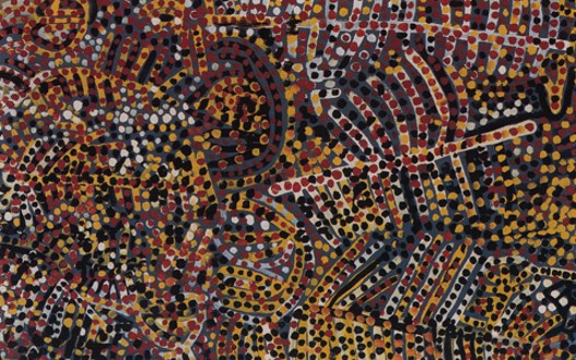
cc <- ochre_palettes$emu_woman_paired[c(6, 11, 2, 7, 9)] %>% 
  rep(5)

tibble::tibble(
  fixed_radius = n + 2,
  cycling_radius = 1:n,
  pen_radius = 1:n + 0,
  transparency = 0.85,
  rotation = pi / 6,
  colors = cc,
  file = paste0("asdf", 1:n, ".svg")) %>%
  purrr::pmap(spiro) %>%
  image_merge(
    output = "emu_woman_sunset.svg") %>%
  image_scale(scale = seq(1, 0.1, length.out = n) ^ 0.85)

Color palette selected from Emily Kngwarreye’s Emu Woman (1988)

When Time Reverses,
You’ll Know What’s Coming

spiro(
  fixed_radius = 919,
  cycling_radius = 367,
  pen_radius = 509,
  windings = 403,
  color_groups = 17,
  color_cycles = 6,
  points_per_polygon = 500,
  transparency = 0.5,
  file = "when_time_reverses.svg",
  colors = scico(17, palette = "tofino")
)

Purple Midnight

spiro(
  file = "purple_midnight.svg",
  fixed_radius = 800,
  cycling_radius = 751,
  pen_radius = 40,
  color_groups = 4,
  color_cycles = 2,
  points_per_polygon = 5000,
  colors = c(
    "midnightblue", 
    "white", 
    "purple4", 
    "white")) %>%
  add_lines(
    colors = "black",
    line_width = 0.15) %>%
  add_background_gradient(
    stops = c(0,0.25,0.63,0.67,0.70,1),
    colors = c(
      "black",
      "purple4", 
      "black",
      "midnightblue", 
      "black", 
      "gray20")) 

Skyscraper Sunrise

set.seed(365)

k <- 12
bg_colors <- scico(31, palette = "vik") %>% 
  rev() %>% 
  scales::muted(., l = 7, c = 7) %>% 
  `[`(sample(1:31, k, replace = T))

bg_stops <- sort(runif(k))
spiro(
  fixed_radius = 1231,
  cycling_radius = 529,
  pen_radius = 1233,
  color_groups = 67,
  color_cycles = 59,
  windings = 101,
  points_per_polygon = 100,
  transparency = 1,
  colors = rev(scico(67, palette = "vik")),
  file = "skyscraper_sunrise.svg") %>%
  add_background_gradient(bg_colors, stops = bg_stops)

k <- 80
  spiro(3,1,0.5,
    file = "asdf.svg",
    color_groups = 3,
    transparency = 0.5,
    colors = c("#AC1014", "#C0C0C0", "#175C02"),
    points_per_polygon = 100) %>%
    image_merge(
      copies = k,
      output = "counterspin_triangles.svg") %>%
    image_scale(scale = seq(1, 0.1, length.out = k)) %>%
    image_spin(rpm = rep(c(1, -1), k / 2) * seq(1, 3, length.out = k)) %>%
    add_background(rounding = 1) %>% 
    add_restart()

Illusively Elusive Allusion

k <- 80
  spiro(
    4,
    3,
    3,
    file = "asdf.svg",
    color_groups = 4,
    colors = rgb(
      c(0, .1418, .2118, .7012),
      c(.0039, .1608, .6392, 1),
      c(.3059, 0.9569, .9922, .9647),
    )  ,
    transparency = 0.5,
    points_per_polygon = 100
  ) %>%
    image_merge(
      copies = k,
      output = "illusively_elusive_allusion.svg") %>%
    image_scale(scale = seq(1, 0.2, length.out = k)) %>%
    image_spin(rpm = rep(c(1, -1), k / 2) * seq(1, 10, length.out = k)) %>% 
  add_restart()

Blurry Metal Eye

spiro(
  fixed_radius = 167,
  cycling_radius = 173,
  pen_radius = 14,
  windings = 173,
  color_groups = 52,
  color_cycles = 72 ,
  points_per_polygon = 50,
  file = "blurry_eye.svg",
  colors = scico(
    n = 52,
    alpha = 0.9,
    palette = "roma")) %>%
  image_merge(
    copies = 6,
    output = "blurry_metal_eye.svg") %>%
  image_scale(seq(1, 0.95, length.out = 6)) %>%
  add_background(rounding = 1)

Maelstrom Sunset

spiro(
  fixed_radius = 12 ,
  cycling_radius = 121, 
  pen_radius = 100,
  file = "maelstrom_sunset.svg", 
  color_groups = 36,
  color_cycles = 48, 
  points_per_polygon = 400,
  colors = scico(18,palette = "roma")) %>% 
  add_background(rounding = 0)

Can We Open It, Grandma?

c(spiro(
  fixed_radius = 21,
  cycling_radius = -20,
  pen_radius = 35,
  transparency = 0.2,
  colors = "black",
  file = "not_forgotten1.svg") %>% 
  add_lines(colors = "#FFFFFFAA", line_width = .25),
  spiro(
  fixed_radius = 21,
  cycling_radius = -20,
  pen_radius = 35,
  transparency = .75,
  colors = "black",
  rotation = pi / 21,
  file = "not_forgotten2.svg") %>% 
  add_lines(colors = "#FFFFFFAA", line_width = .5)) %>%
  image_merge(output = "not_forgotten.svg") %>% 
  add_background_gradient(
    rounding = 1, 
    radius = 1,
    colors = c("lightcyan2",
      rep(c("royalblue4", "lightcyan2"), 13),"royalblue4",
      rep("white",2)),
      stops = c(0,
        0.05, 0.07, 
        0.11, 0.1578947, 
        0.2105263, 0.28, 
        0.3395, 0.39, 
        0.441, 0.485, 
        0.53, 0.571, 
        0.609, 0.6415, 
        0.682, 0.711, 
        0.745, 0.77, 
        0.80, 0.823, 
        0.84, 0.86, 
        0.88, 0.895, 
        0.905, 0.91, 
        0.92, 0.93, 1))

D’Ya Wanna Roller Skate?

k <- 40
tibble(
  fixed_radius = 5,
  cycling_radius = 3,
  pen_radius = seq(12, 3, length.out = k),
  colors = viridis::viridis(k, option = "D", alpha = 0.15),
  rotation = seq(5 * pi / k,0,  length.out = k)) %>%
  pmap_chr(spiro) %>%
  image_merge(
    output = "wanna_rollerskate.svg") %>%
  image_rotate(degrees = -360 / 20) %>%
  # image_spin(1:k / k) %>%
  add_background()

Checkered Future

ngroups <- 4 * 6

cc <- c(
  rainbow(ngroups / 4, s = 0.9, v = 0.3),
  rev(rainbow(ngroups / 4, s = 0.9, v = 0.3)),
  rainbow(ngroups / 4, s = 0.3, v = .9),
  rev(rainbow(ngroups / 4, s = 0.3, v = .9)))
  
cc[seq(2, ngroups, 2)] <- "black"
  
spiro(
  fixed_radius = 199,
  cycling_radius = 120,
  pen_radius = 43,
  color_groups = ngroups,
  color_cycles = 1440 %/% ngroups,
  points_per_polygon = 100,
  transparency = .3,
  draw_fills = T,
  colors = cc,
  file = "checkered_future.svg") %>%
  add_background_gradient(
    colors = c(
      "black", "black",
      "gray90", "black",
      "gray95", "black",
      "gray50"),
    stops = c(
      .00, .18,
      .20, .3,
      .50, .60,
      1))

Expensive Plaid

spiro(
  fixed_radius = 1,
  cycling_radius = sqrt(7),
  pen_radius = sqrt(7),
  windings = 450,
  draw_fills = F,
  colors = c(
    scico(11, palette = "tofino", direction = 1),
    scico(4, palette = "nuuk")),
  color_groups = 16,
  points_per_polygon = 100,
  color_cycles = 450 * 8,
  line_width = 0.75,
  lend = 1,
  file = "expensive_plaid.svg") %>%
  add_background()

Groovy Church

cc <- hcl(
  h = seq(0,1,length.out = 52) * 220 + 70, 
  c = 50, 
  l = 28)

cc[1:14] <- hcl(
  h = seq(0,1,length.out = 14) * 250 + 80, 
  c = 60, 
  l = 42)

# cc <- scales::muted(cc, l = 40)
spiro(
  fixed_radius = 44,
  cycling_radius = 13,
  pen_radius = 13,
  file = "asdf.svg",
  colors = cc,
  color_cycles = 4,
  draw_fills = F,
  color_groups = 4 * 13,
  points_per_polygon = 15,
  line_width = 0.3) %>%
  spiro::image_merge(.,
    output = "groovy_church.svg", 
    copies = 38) %>%
  image_rotate(1:36 * 0.21) %>%
  add_background_gradient(
    colors = c("gray15", "black", 
               "black", "gray10", "black",
               "black", "gray15"),
    stops = c(0,0.27,
              0.271, 0.5, .655,
              0.656,1))

Hawaiian Snow Salad

spiro(
  fixed_radius = 200,
  cycling_radius = 89, 
  pen_radius = 175,
  color_groups = 200, 
  color_cycles = 5, 
  points_per_polygon = 1000, 
  file = "hawaiian_snow_salad.svg",
  colors = alpha(lacroix_palette(
    name = "Coconut",
    n = 200,
    type = "continuous"), 
    alpha = 0.8))

Was It This Obvious All Along?

tibble::tibble(
  points_per_polygon = 1000,
  fixed_radius = 17,
  cycling_radius = 3:8,
  colors = c(
    "dodgerblue4", "white",
    "dodgerblue3", "white",
    "dodgerblue2", "white")) %>% 
  pmap_chr(spiro) %>%
  image_merge(
    output = "i_saw_your_movie.svg")

Yes You May

k <- 12

crossing(
  fixed_radius = k,
  cycling_radius = seq(1,k),
  pen_radius = k) %>% 
  rowid_to_column("file") %>%
  mutate(
    file = paste0(file,".svg"),
    colors = c(
      scico(
        n = nrow(.) / 2, 
        palette = "devon", 
        alpha = .9), 
      scico(
        n = nrow(.) / 2, 
        palette = "devon", 
        alpha = .7))) %>% 
  pmap(
    spiro, 
    draw_fills = T) %>% 
  rev() -> p

p[-1:-3] %>% 
  rev %>% 
  map2(
    seq(1,0.5, length.out = length(.)) ^ 0.4 , 
    image_scale) %>%
  image_merge(
    output = "yes_you_may.svg") %>% 
  add_lines(line_width = 0.2) 

The Foreglow of
a Simple Insight

l <- 27
  crossing(
    fixed_radius = 17,
    cycling_radius = 1:9,
    pen_radius = 11
  ) %>%
    mutate(colors = LaCroixColoR::lacroix_palette("Coconut", n =  9) %>% scales::alpha(0.9)) %>%
    pmap(
      spiro,
      draw_fills = T,
      xlim = c(-l, l),
      ylim = c(-l, l),
      color_cycles = 17 * 6,
      points_per_polygon = 500
    ) %>%
    image_merge(output = "foreglow.svg") %>%
    add_background_gradient(
      colors = rep(
        LaCroixColoR::lacroix_palette("Coconut", 9) %>% colorspace::darken(.1),
        3
      ),
      stops = c(0.7 * seq(0, 1, length.out = l - 3), 0.78 , 0.88, 0.98)
    )

Bending Is Not a Compromise

n <- 36

tibble(
  fixed_radius = 13,
  cycling_radius = 11,
  pen_radius = seq(1, n) / 2,
  file = paste0("sp", 1:n, ".svg"),
  colors = rep(scico(
    n = n / 4,
    alpha = 0.6,
    palette = "tofino"),
  times = 4)) %>%
  pmap(spiro,
       xlim = c(-20, 20),
       ylim = c(-20, 20)) %>%
  rev() %>%
  image_merge(
    output = "bending_is_not_a_compromise.svg") %>%
  image_rotate(sqrt(1:n * 50)) %>%
  add_background()

Value-Added Fragility

spiro(
  fixed_radius = 121,
  cycling_radius = 131, 
  pen_radius = 11,
  file = "value_added_fragility.svg", 
  color_groups = 121,
  color_cycles = 11, 
  points_per_polygon = 100,
  colors = scico(11,palette = "cork")) %>% 
  add_background(rounding = 0)

Restoration Agreement

c(
  spiro(
      file = "restoration_agreement1.svg",
      fixed_radius = 800,
      cycling_radius = 677,
      pen_radius = 101,
      color_groups = 8,
      color_cycles = 677 * 3 ,
      windings = 677 * 0.5,
      transparency = 1,
      rotation = pi / 13,
      points_per_polygon = 3,
      colors = paste0("gray", c(92,93,94,95,12,13,14,15))
    ),
  spiro(
    file = "restoration_agreement2.svg",
    fixed_radius = 800,
    cycling_radius = 677,
    pen_radius = 101,
    color_groups = 8,
    color_cycles = 677 * 3 ,
    windings = 677 * 0.5,
    transparency = 1,
    points_per_polygon = 3,
    colors = scico(n = 8, palette = "cork")
  )) %>% 
  image_merge(output = "restoration_agreement.svg") %>%
  add_background(color = "gray8")

Reconciliation Reset 490

n <- 36
spiro(fixed_radius = 3,
      cycling_radius = 1, 
      file = "reconciliation491.svg", 
      colors = "#5262CA10", 
      points_per_polygon = 300) %>% 
  image_scale(scale = 0.7) %>% 
  image_merge(copies = n, 
              output = "reconciliation491.svg") %>% 
  add_lines(colors = "#5262CAAA", line_width = 0.5) %>% 
  image_spin(rpm = seq(1,n) / 12, 
             rotation_point = c(0.6135,0.6135)) %>% 
  image_shift(x = -81.5, y = 81.5) %>%
  add_restart(color = colorspace::lighten("#5262CA", .5), 
              fill = colorspace::darken("#5262CA", .85)) %>% 
  add_background_gradient(colors = map(c(0.98, 0.98, 0.95, 0.8), 
                                       colorspace::darken, 
                                       col = "#5262CA")) 

Convoluted Candor

lim <- 5
k <- 36
tibble(
  pen_radius = seq(3, 1, length.out = k),
  colors = scico(n = k, palette = "cork") %>% 
    scales::muted(., l = 50, c = 40),
  transparency = rep_len(c(rep(0.4, 3), 1), k),
  line_width = rep_len(c(rep(0.5, 3), 1), k)
) %>%
  pmap(
    spiro,
    fixed_radius = 5,
    cycling_radius = 3,
    rotation = -pi / 2,
    xlim = c(-lim, lim),
    ylim = c(-lim, lim),
    draw_fill = F
  ) %>%
  image_merge("convoluted_candor.svg", delete_input = T)

Epistemological Modesty

spiro(
  fixed_radius = 8,
  cycling_radius = 7,
  pen_radius = 1.069,
  color_groups = 8,
  color_cycles = 2,
  start_angle = 0,
  rotation = -pi / 8 ,
  transparency = .5,
  points_per_polygon = 5000,
  windings = 7 * 6,
  file = "epistemological_modesty.svg",
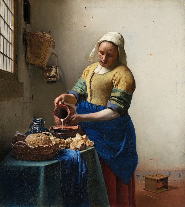
  colors = dutchmasters_pal(
    palette = "milkmaid",
    reverse = T)(8))

Color palette selected from Vermeer’s Milkmaid

Happy Birthday,
Whenever It Was

spiro(
  fixed_radius = sqrt(13),
  cycling_radius = sqrt(11),
  pen_radius = sqrt(0.5), 
  windings = 401, 
  color_groups = 5, 
  points_per_polygon = 40, 
  color_cycles = 906,
  colors = c("darkred","gray90","darkgreen","gray20","forestgreen"), 
  transparency = 0.55, 
  file = "christmas_wreath.svg") %>% 
  add_background_gradient(
    rounding = 1,
    radius = 1, 
    colors = c("white",rep(c("gray30","black"), 5),"white"), 
    stops = c(0.4,seq(.45,.9,length.out = 10),0.93))

Web Windows

n <- 10
spiro(
  fixed_radius = 6,
  cycling_radius = 11,
  pen_radius = -6 ,
  colors = "white",
  file = "web_windows.svg",
  draw_fills = F,
  transparency = 0.9,
  line_width = 0.75,
  rotation = pi / 6,
  points_per_polygon = 1000) %>%
  image_merge(
    output = "web_windows.svg",
    copies = n) %>%
  add_fills(viridis_pal(
    end = 0.97,
    alpha = 0.9)(n)) %>%
  image_scale(scale = 1.07 * sqrt(0.8 ^ (seq(0, n - 1)))) %>%
  image_spin(rpm = 1:n * 0.15) %>% 
  add_restart(
    fill = "#00000000",
    color = "white",
    ) %>%
  add_background()

Colliding Scopes

tibble(colors = c("#004D47", "#128277")) %>%
  pmap(
    spiro,
    fixed_radius = pi,
    cycling_radius = sqrt(8),
    pen_radius = 0.5 * sqrt(8) / pi,
    windings = 81,
    start_angle = 0,
    points_per_polygon = 40001,
    transparency = 1) %>%
  tibble(
    input = ., 
    duration = c(7, 11)) %>% 
  pmap(image_animate,
     attribute = "opacity",
     values = c(0.2, 0.8, 0.2)) %>% 
  image_merge(
  output = "colliding_scopes.svg",
  delete_input = T) %>%
  image_spin(rpm = c(0.1,-0.1)) %>% 
  add_restart()

The Increasing Returns
of Having Traveled

n <- 60
spiro(3, 1, 1, 
      color_groups = 6, 
      colors =  LaCroixColoR::lacroix_palettes$Tangerine[1,, drop = T] %>% 
        scales::alpha(0.7), 
      file = "delta.svg") %>% 
  image_merge(copies = n, 
              output = "the_increasing_returns_of_having_travelled.svg") %>% 
  image_scale(seq(0.0001,1, length.out = n) ^ (1/1.25)) %>% 
  image_rotate(seq(0,360 * 5.65, length.out = n)) %>% 
  spiro::add_lines(input = ., colors = "gray10") %>% 
  add_background_gradient(colors = c("gray30", "gray5","gray30","gray5"))

Mining Old Errors
for New Truths

my_palette <-
  scales::colour_ramp(c(
    rgb(.74, .19, .22, .9),
    rgb(.86, .76, .22, .2),
    rgb(.91, .92, .92, .9),
    rgb(.11, .22, .22, .95),
    rgb(.22, .22, .22, .1),
    rgb(.24, .22, .71, .9)
  ))
spiro(
  fixed_radius = 226,
  pen_radius = 235,
  cycling_radius = 15,
  points_per_polygon = 10,
  file = "old_errors.svg",
  color_groups = 40,
  color_cycles = 61,
  colors = my_palette(seq(0, 1, length.out = 40)) 
) %>% 
  add_background_gradient(colors = c("gray20", "white", "gray90", "gray30","gray5"), 
                          stops = c(0, .1, 0.6, .65, 1))

Ñañaras

my_colors <- c("#969594FF","#00000000","#00000000",
               "#F9F8F7FF","#00000000","#00000000",
               "#585756FF","#00000000","#00000000",
               "#D0CFCDFF","#00000000","#00000000","#171615FF")

tibble(fixed_radius = 541,
       cycling_radius = 601,
       pen_radius = 191, 
       windings = 200,
       color_groups = 20,
       points_per_polygon = 40 * 19:23) %>% 
  pmap(spiro, colors = my_colors) %>% 
  image_merge(output = "nanaras.svg") %>% 
  image_scale(c(1.07, .56, .29, 0.15, 0.075)) %>% 
  image_rotate(degrees = seq(0, 80, 20)) %>% 
  add_background("black")

The Past Was Never Simple

spiro(
  fixed_radius = 800,
  cycling_radius = 749,
  pen_radius = 51,
  color_groups = 4,
  color_cycles = 2,
  transparency = 0.25,
  start_angle = 0,
  points_per_polygon = 10000,
  rotation = -pi / 8,
  windings = 749,
  file = "the_past_was_never_simple.svg",
  colors = c(
    "firebrick4",
    "purple4",
    "midnightblue",
    "black")) %>%
  add_background_gradient(
    rounding = 0,
    stops = c(0, .08, 0.083, .6, 0.7, 1),
    colors = c(
      "white", 
      "gray95", 
      "gray40", 
      "white", 
      "white", 
      "white"))

Portal to the 80s

string_bezier(
  file = "portal_to_the_80s.svg",
  x = c(-1, 1, 0,-1, 1,-1, 0, 1,-1, 1),
  y = c(0, 0, 1, 0, 0, 0,-1, 0, 0, 0),
  color = c("#006B6B", "#FFFFFF", "black", "black", "black"),
  n = 200,
  lwd = 5,
  ljoin = 1) %>%
  add_background(color = "#108998")

Non-spirograph string art with Bézier curves

Supervillains’ Superior
Sense of Fashion

library(ggforce)

k <- 30
r <- rep(0, k)
r[1:2] <- 1
for (i in 3:k) {
  r[i] <- r[i - 1] * 1 / cos(pi / i)
}
xy <- function(n, r, dtheta) {
  tibble(x = r * cos((0:n) * dtheta + pi / 2),
         y = r * sin((0:n) * dtheta + pi / 2))
}


svg("superhero.svg", width = 8, height = 8)
par(pty = "s")
k <- 30
r <- rep(0, k)
r[1:2] <- 1
for (i in 3:k) {
  r[i] <- r[i - 1] * 1 / cos(pi / i)
}
plot(
  x = c(1, 2),
  y = c(1, 2),
  xlim = c(-8.7, 8.7),
  ylim = c(-8.7, 8.7),
  type = "n",
  axes = F,
  xlab = NA,
  ylab = NA,
  ann = F
)

bg <- "slateblue"
plotrix::draw.circle(
  0,
  0,
  radius = 8.7,
  col = bg,
  border = NA,
  nv = 200
)
tibble(n = 2:k, r = r[-1]) %>%
  mutate(dtheta = 2 * pi / n,
         d_xy = pmap(list(n, r, dtheta), xy)) %>%
  select(-dtheta) %>%
  arrange(-n) %>%
  purrr::pwalk(., function(n, r, d_xy) {
    plotrix::draw.circle(
      0,
      0,
      radius = r,
      col = paste0("gray", n * 3),
      border = bg,
      lwd = 2 * (2 / n) ^ (1 / 5),
      nv = 200
    )
    if (n > 2)
      polygon(
        d_xy,
        col = paste0("gray", 2),
        border = bg,
        lwd
        = 2 * (2 / n) ^ (1 / 5)
      )
  })
dev.off()

Inscribed polygons adapted from Mathologer’s T-Shirt.

One-Minute Reunion

spiro(
  fixed_radius = 5,
  cycling_radius = 1,
  pen_radius = 11 / 3,
  color_groups = 5,
  colors = rep("gray95", 5),
  start_angle = pi,
  draw_fills = FALSE,
  rotation = pi / 10,
  file = "one_minute_reunion.svg",
  points_per_polygon = 250) %>% 
  add_pathdot(
    colors = "firebrick", 
    duration = c(2,3,4,5,6,10,12,15,20,30,60)) %>% 
  # add_restart(color = "#333333",fill = scales::alpha("gray95")) %>% 
  add_background("gray95")

When Ryan was learning about Least Common Multiples, he asked me if I ever used them outside of a math class. Here ya go, buddy!
What is the least common multiple of 2, 3, 4, 5, 6, 10, 12, 15, 20, 30, and 60?

Sunrises Are Sunsets Recycled

k <- 9
n_dots <- 120
cc <- lacroix_palette(
  name = "Coconut", 
  n = n_dots) %>% 
  alpha(0.7)

s <- spiro(
  fixed_radius = 9,
  cycling_radius =     4,
  pen_radius =     6,
  draw_fills = F,
  colors = alpha(rep("black", k), 0.01),
  color_groups = k,
  points_per_polygon = 50,
  file = "asdf.svg")

for (i in seq(0, n_dots - 1)) {
  s <- add_pathdot(
    s,
    delay = i / (n_dots / 12),
    colors = cc[i + 1],
    radius = 2,
    duration = 32)
}
  
image_merge(
  s,
  copies = 5, 
  output = "sunrises_are_sunsets_recycled.svg") %>%
  image_spin(rpm = 1:5 / 5) %>%
  add_restart(color = "white", fill = "black") %>%
  add_background()

Graceful Exit

tibble(
  cycling_radius = c(-5,5),
  color_cycles = c(64,32),
  start_angle = c(0 * pi / 64 * 3, 20 * pi / 8),
  line_width = c(4 * 0.68, 4),
  file = c("s3.svg","s4.svg")) %>% 
  pmap(
    spiro,
    fixed_radius = 8,
    pen_radius = 5,
    color_groups = 64,
    points_per_polygon = 2,
    draw_fills = F,
    ljoin = 2,
    end_at_beginning = T,
    colors = c(
      viridis_pal()(32),
      rev(viridis_pal()(32)))) %>% 
  tibble(input = ., scale = c(1,0.68)) %>% 
  pmap(image_scale) %>% 
  image_merge(
    output = "graceful_exit.svg", 
    delete_input = T) %>%
  add_background_gradient(colors = c("gray5", "gray25"))