To investigate causal relations, experiments with manipulated variables are the most straightforward and persuasive forms of evidence we have. Unfortunately, there are a lot of interesting variables that are hard to manipulate experimentally. To investigate what they cause and what causes such variables, longitudinal studies are among the most useful forms of evidence we have.

For example, reading comprehension and vocabulary have a reciprocally causal relationship (Killingly et al., 2025; Quinn et al., 2015). That is, if you have a good vocabulary, it is easier for you to comprehend text. If it is easy for you to comprehend text, you will likely expand your vocabulary.

Killingly, C., Graham, L. J., Tancredi, H., & Snow, P. (2025). Reciprocal relationships among reading and vocabulary over time: A longitudinal study from grade 1 to 5. Reading and Writing, 38(3), 605–625. https://doi.org/10.1007/s11145-024-10522-x

Quinn, J. M., Wagner, R. K., Petscher, Y., & Lopez, D. (2015). Developmental relations between vocabulary knowledge and reading comprehension: A latent change score modeling study. Child Development, 86(1), 159–175. https://doi.org/10.1111/cdev.12292

Unfortunately, many of our initial methods of understanding longitudinal relationships can generate misleading findings.

Cross-Lag Panel Models (CLPM)

One intuitively simple model is the cross-lagged panel model, as shown with four time periods in Figure 1. The cross-lag panel model has two series of variables, X and Y. The paths within each series (X₁ to X₂ to X₃ to X₄ and Y₁ to Y₂ to Y₃ to Y₄) are called auto-regressive paths, meaning that each variable is predicting itself across time.

Each variable also influences the other at a subsequent time. These paths crossing from one series to the other are called cross lags.

In addition to the cross lags and autoregressive paths, the series have correlated errors, which allow variables measured at the same time to have additional reasons to correlate.

Code

my_observed <- redefault(ob_ellipse, m1 = 15)
my_connect <- redefault(connect, resect = 2)
my_error <- redefault(ob_circle, radius = .35)
my_font <- "Roboto Condensed"
k <- 4
my_sep <- 4
ggdiagram(font_family = my_font, font_size = 24) +
  {x <- my_observed() %>% 
    ob_array(k, sep = my_sep, 
             where = "south", 
             label = paste0("*X*~" , 1:k, "~"))} +
  {y <- my_observed(label = paste0("*Y*~" ,1:k, "~")) %>%  
    place(x, "right", sep = my_sep)} +
  {e_x <- my_error() %>% place(x[-1], "right", sep = .6)} +
  {e_y <- my_error() %>% place(y[-1], "left", sep = .6)} +
  my_connect(x[-k], x[-1], 
             label = ob_label("*b*~*XX*~", 
                              angle = 0, 
                              size = 12)) +
  my_connect(x[-k], y[-1], 
             label = ob_label("*b*~*XY*~", 
                              angle = 0, 
                              size = 12, position = .27)) +
  my_connect(y[-k], x[-1], 
             label = ob_label("*b*~*YX*~", 
                              angle = 0, 
                              size = 12, position = .27)) +
  my_connect(y[-k], y[-1], 
             label = ob_label("*b*~*YY*~", 
                              angle = 0, 
                              size = 12)) + 
  my_connect(e_x, x[-1], length_head = 5, resect = 1) + 
  my_connect(e_y, y[-1], length_head = 5, resect = 1) +
  {tau_x1y1 <- ob_covariance(x[1], y[1])} +
  ob_latex("\\tau_{X_1Y_1}", tau_x1y1@midpoint(), width = 1.35, delete_files = F, force_recompile = F) +
  {tau_xy <- ob_covariance(e_y, e_x, 
                resect = 1, 
                length_head = 4, 
                length_fins = 4, 
                looseness = 1.3)} + 
  ob_latex("\\tau_{xy}", tau_xy@midpoint(), width = .95, delete_files = F, force_recompile = T) +
  {tau_x2 <- ob_variance(x[1], 
              length_head = 5, 
              length_fins = 5, 
              resect = 1, 
              bend = -10, 
              theta = degree(65), 
              looseness = 1.1)} + 
  ob_latex("\\tau^2_{X_1}", tau_x2@midpoint(), width = .85, delete_files = F, force_recompile = F) +
  {tau_y2 <- ob_variance(y[1], 
              length_head = 5, 
              length_fins = 5, 
              resect = 1, 
              bend = degree(-10), 
              theta = degree(65), 
              looseness = 1.1)} +
  ob_latex("\\tau^2_{Y_1}", tau_y2@midpoint(), width = .85, delete_files = F, force_recompile = F) +
  {tau_ex2 <- ob_variance(e_x, 
              length_head = 5, 
              length_fins = 5, 
              resect = 1, 
              # bend = degree(-90), 
              theta = degree(90), 
              looseness = 3.5)} +
  ob_latex("\\tau^2_{X}", tau_ex2@midpoint(), width = .75, force_recompile = F, delete_files = F) +
  {tau_ey2 <- ob_variance(e_y, 
              length_head = 5, 
              length_fins = 5, 
              resect = 1, 
              # bend = degree(-90), 
              theta = degree(90), 
              looseness = 3.5)} +
  ob_latex("\\tau^2_{Y}", tau_ey2@midpoint(), width = .75, delete_files = F, force_recompile = F)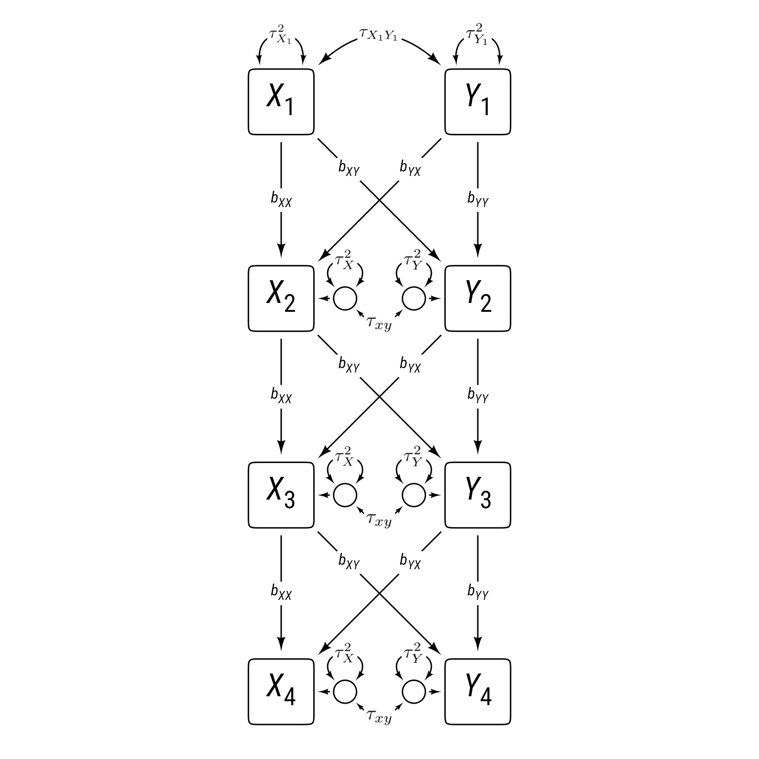

Automating repetitive lavaan models

Unfortunately, lavaan models can become quite large. In most lavaan models, we do not need to name the parameters. However, if we are specifying parameters are constrained to equal each other, we need to name our parameters. Any parameter with the same name is constrained to be equal.

To specify the model with lavaan syntax, one could do it by hand like so:

m <- '
# Covariances
x1 ~~ tau_x1 * x1
y1 ~~ tau_y1 * y1 + tau_x1y1 * x1
x2 ~~ tau_xx * x2 + tau_xy * y2 
x3 ~~ tau_xx * x3 + tau_xy * y3
x4 ~~ tau_xx * x4 + tau_xy * y4
y2 ~~ tau_yy * y2 
y3 ~~ tau_yy * y3
y4 ~~ tau_yy * y4
# Regressions with intercepts
x1 ~ b_x01 * 1
x2 ~ b_x02 * 1 + b_xx * x1 + b_yx * y1
x3 ~ b_x03 * 1 + b_xx * x2 + b_yx * y2
x4 ~ b_x04 * 1 + b_xx * x3 + b_yx * y3
y1 ~ b_y01 * 1
y2 ~ b_y02 * 1 + b_yy * y1 + b_xy * x1
y3 ~ b_y03 * 1 + b_yy * y2 + b_xy * x2
y4 ~ b_y04 * 1 + b_yy * y3 + b_xy * x3
'

The benefits of this approach are that the code is easier to create and to understand. With only 4 waves of data, this model does not seem so difficult to specify by hand.

The liabilities of this approach are that it is error prone and increasingly tedious for large models. We are better off using paste0 or glue from the glue package to automate model production.

Pasting text together with `paste0`

The paste0 function is a special variant of the paste function that has 0 separation between the pasted elements. By default, paste separates the elements with spaces:

paste("A", "B", "C")

[1] "A B C"

You can put anything between the elements with the sep parameter:

paste("A", "B", "C", sep = ",")

[1] "A,B,C"

The paste0 function pastes text together. For example,

paste0("A", "B", "C")

[1] "ABC"

If you use a vector, paste0 will paste multiple strings:

paste0("A", 1:3)

[1] "A1" "A2" "A3"

We can “collapse” the vector strings into a single string separated by the newline symbol \n:

paste0("A", 1:3, collapse = "\n") %>% 
  cat()

A1
A2
A3

Pasting repetitive code

Suppose we have 8 waves of data. We need to set the variances of the x series.

This is what we need:

x1 ~~ tau_x1 * x1 
x2 ~~ tau_xx * x2 
x3 ~~ tau_xx * x3 
x4 ~~ tau_xx * x4 
x5 ~~ tau_xx * x5 
x6 ~~ tau_xx * x6
x7 ~~ tau_xx * x7 
x8 ~~ tau_xx * x8

We see that each line is very similar. We need to create vectors for the parts that change: the numbers 1 to 8 and the variance parameters (tau_x1 and tau_xx). The numbers 1 to 8 are easy to make with the : operator.

1:8

[1] 1 2 3 4 5 6 7 8

Alternately, we could use the seq function to make a sequence:

seq(1, 8)

[1] 1 2 3 4 5 6 7 8

However, we do not want our code to be tied specifically to the number 8. We want any number of waves. We define a variable k for the number of waves and make a sequence

k <- 8
1:k

[1] 1 2 3 4 5 6 7 8

# or
seq(1, k)

[1] 1 2 3 4 5 6 7 8

# or omit the start value
seq(k)

[1] 1 2 3 4 5 6 7 8

The variance parameters are all the same except for x1. So we need a vector that is one value for the first element and repeated k - 1 times for the remaining elements. The rep function repeats elements as many times as you specify:

rep("tau_xx", k - 1)

[1] "tau_xx" "tau_xx" "tau_xx" "tau_xx" "tau_xx" "tau_xx" "tau_xx"

Putting the first and remaining elements together:

v_x <- c("tau_x1", rep("tau_xx", k - 1))
v_x

[1] "tau_x1" "tau_xx" "tau_xx" "tau_xx" "tau_xx" "tau_xx" "tau_xx" "tau_xx"

Now we are ready to paste the entire line of code:

# Make string
var_x <- paste0("x", 1:k, " ~~ ", v_x, " * x", 1:k, collapse = "\n") 

# Output string 
cat(var_x)

x1 ~~ tau_x1 * x1
x2 ~~ tau_xx * x2
x3 ~~ tau_xx * x3
x4 ~~ tau_xx * x4
x5 ~~ tau_xx * x5
x6 ~~ tau_xx * x6
x7 ~~ tau_xx * x7
x8 ~~ tau_xx * x8

The `glue` function: An alternative to `paste0`

Many people find the glue function from the glue package easier to read than the paste0 function. Put everything inside a single string, with R code enclosed in curly braces:

library(glue)
var_x <- glue("x{1:k} ~~ {v_x} * x{1:k}")

The glue_collapse function is useful to see the output of glue as one string:

glue_collapse(var_x, sep = "\n")

x1 ~~ tau_x1 * x1
x2 ~~ tau_xx * x2
x3 ~~ tau_xx * x3
x4 ~~ tau_xx * x4
x5 ~~ tau_xx * x5
x6 ~~ tau_xx * x6
x7 ~~ tau_xx * x7
x8 ~~ tau_xx * x8

Specifying the CLPM Model

To specify Figure 1 with automated lavaan syntax

library(glue)
# Number of waves
k <- 4
# Sequence from 2 to k
s2k <- seq(2, k)
# Sequence from 1 to k - 1
s1k1 <- seq(1, k - 1)

# variance symbols for x
v_x <- c("tau_x1", rep("tau_xx", k - 1))
# variance symbols for y
v_y <- c("tau_y1", rep("tau_yy", k - 1))
# covariance symbols xy
cov_xy <- c("tau_x1y1", rep("tau_xy", k - 1))


# Model with comments added
m_clpm <- c(
  "# Regressions",
  glue("x{s2k} ~ b_xx * x{s1k1} + b_yx * y{s1k1}"),
  glue("y{s2k} ~ b_yy * y{s1k1} + b_xy * x{s1k1}") ,
  "# Variances",
  glue("x{1:k} ~~ {v_x} * x{1:k}"),
  glue("y{1:k} ~~ {v_y} * y{1:k}"),
  "# Covariances",
  glue("x{1:k} ~~ {cov_xy} * y{1:k}"),
  "# Intercepts",
  glue("x{1:k} ~ b_x0{1:k} * 1"),
  glue("y{1:k} ~ b_y0{1:k} * 1")
) %>%
  glue_collapse("\n")

m_clpm

# Regressions
x2 ~ b_xx * x1 + b_yx * y1
x3 ~ b_xx * x2 + b_yx * y2
x4 ~ b_xx * x3 + b_yx * y3
y2 ~ b_yy * y1 + b_xy * x1
y3 ~ b_yy * y2 + b_xy * x2
y4 ~ b_yy * y3 + b_xy * x3
# Variances
x1 ~~ tau_x1 * x1
x2 ~~ tau_xx * x2
x3 ~~ tau_xx * x3
x4 ~~ tau_xx * x4
y1 ~~ tau_y1 * y1
y2 ~~ tau_yy * y2
y3 ~~ tau_yy * y3
y4 ~~ tau_yy * y4
# Covariances
x1 ~~ tau_x1y1 * y1
x2 ~~ tau_xy * y2
x3 ~~ tau_xy * y3
x4 ~~ tau_xy * y4
# Intercepts
x1 ~ b_x01 * 1
x2 ~ b_x02 * 1
x3 ~ b_x03 * 1
x4 ~ b_x04 * 1
y1 ~ b_y01 * 1
y2 ~ b_y02 * 1
y3 ~ b_y03 * 1
y4 ~ b_y04 * 1

Simulating data based on the CLPM

To simulate data, we need to replace the parameter labels in the model with specific values. Doing so by hand is no fun, and it is easy to mess things up when playing with different values. I recommend placing parameter labels programmatically with a named vector and a custom function.

Here is a named vector of parameter values:

my_parameters <- c(
  tau_xx = .4,
  tau_yy = .5,
  tau_x1y1 = .4,
  tau_xy = .2,
  tau_x1 = 1,
  tau_y1 = 1,
  b_xx = .7,
  b_yy = .6,
  b_xy = 0,
  b_yx = 0.3
)

I have made a custom function replace_parametersto replace parameter labels. I have also made a custom function plot_cor to plot correlation matrices.

replace_parameters <- function(model, params) {
  # Make sure replacements are whole words
  names(params) <- paste0("\\b", names(params), "\\b")
  # Convert to strings but retain names
  p <- purrr::map_chr(params, as.character)
  # replace all strings
  stringr::str_replace_all(model, p)
}

plot_cor <- function(d, font_size = 16) {
  cor(d) %>%
    corrr::as_cordf(1) %>%
    corrr::stretch() %>%
    mutate(y = fct_rev(y)) %>%
    ggplot(aes(x, y)) +
    geom_tile(aes(fill = r)) +
    geom_text(aes(label = ggdiagram::round_probability(r)), 
              size = font_size * .8, 
              size.unit = "pt") +
    scale_fill_gradient2(NULL,
      limits = c(-1, 1),
      low = "darkgreen",
      mid = "white",
      high = "orchid4",
      breaks = seq(-1, 1, .2),
      labels = \(x) ggdiagram::round_probability(x, digits = 1)
    ) +
    scale_x_discrete(NULL, expand = expansion()) +
    scale_y_discrete(NULL, expand = expansion()) +
    coord_fixed() +
    theme_minimal(base_size = font_size) +
    theme(legend.key.height = unit(1, "null"), 
          legend.text = element_text(hjust = 1), 
          legend.text.position = "left")
}

Let’s make a model to simulate values:

m_clpm_sim <- m_clpm %>% 
  replace_parameters(my_parameters) %>% 
  glue_collapse("\n")

m_clpm_sim

# Regressions
x2 ~ 0.7 * x1 + 0.3 * y1
x3 ~ 0.7 * x2 + 0.3 * y2
x4 ~ 0.7 * x3 + 0.3 * y3
y2 ~ 0.6 * y1 + 0 * x1
y3 ~ 0.6 * y2 + 0 * x2
y4 ~ 0.6 * y3 + 0 * x3
# Variances
x1 ~~ 1 * x1
x2 ~~ 0.4 * x2
x3 ~~ 0.4 * x3
x4 ~~ 0.4 * x4
y1 ~~ 1 * y1
y2 ~~ 0.5 * y2
y3 ~~ 0.5 * y3
y4 ~~ 0.5 * y4
# Covariances
x1 ~~ 0.4 * y1
x2 ~~ 0.2 * y2
x3 ~~ 0.2 * y3
x4 ~~ 0.2 * y4
# Intercepts
x1 ~ b_x01 * 1
x2 ~ b_x02 * 1
x3 ~ b_x03 * 1
x4 ~ b_x04 * 1
y1 ~ b_y01 * 1
y2 ~ b_y02 * 1
y3 ~ b_y03 * 1
y4 ~ b_y04 * 1

Let’s make data that conforms to this model:

d_clpm <- simulateData(model = m_clpm_sim, sample.nobs = 1000)
head(d_clpm)

           x2         x3         x4         y2         y3          y4
1 -0.02513524 -0.5515860 -0.3459570 -0.4127451 -1.1519481 -0.25031330
2 -1.38802737 -0.8563255 -1.3730245 -0.6139934  0.2750190  0.58912670
3 -0.63543548 -0.3448398  0.1147905 -0.8517809 -0.4163680  0.07433635
4  1.26446765  1.3199914  1.5823441  1.5906017  1.5513886  0.02420739
5 -0.79890268 -0.5447566 -0.8385079 -1.4847547  0.1248847 -0.31389952
6 -1.27005260 -3.4041828 -3.6039819 -0.5920997 -1.6813207 -1.17111918
           x1          y1
1  0.28225925 -0.79232876
2 -2.06897472 -1.20090111
3  0.25134607 -0.07389873
4  1.08943815  2.35761335
5 -0.01205474 -2.08521002
6 -1.42854518 -0.37556543

Figure 2 displays the correlations among the variables we have simulated. Notice that adjacent variables are more highly correlated than variables separated by time.

plot_cor(d_clpm)

If we test the free-parameter model on the simulated data, we can see that the estimates are close to the specified population parameters, which increases our confidence that the simulation is correct.

fit_clpm <- sem(model = m_clpm, data = d_clpm) 
my_metrics <- c("Chi2", "Chi2_df", "p_Chi2", "RMSEA", "GFI", "NNFI")
model_performance(fit_clpm, metrics = my_metrics) %>% 
  print_md()

Chi2(26)	p (Chi2)	RMSEA	GFI	NNFI
36.51	0.083	0.02	0.99	1.00

Indices of model performance

model_parameters(fit_clpm, component = "all") %>% 
  print_md()

Link	Coefficient	SE	95% CI	z	p
x2 ~ x1 (b_xx)	0.69	0.01	(0.67, 0.72)	53.43	< .001
x2 ~ y1 (b_yx)	0.32	0.01	(0.29, 0.35)	21.91	< .001
x3 ~ x2 (b_xx)	0.69	0.01	(0.67, 0.72)	53.43	< .001
x3 ~ y2 (b_yx)	0.32	0.01	(0.29, 0.35)	21.91	< .001
x4 ~ x3 (b_xx)	0.69	0.01	(0.67, 0.72)	53.43	< .001
x4 ~ y3 (b_yx)	0.32	0.01	(0.29, 0.35)	21.91	< .001
y2 ~ y1 (b_yy)	0.64	0.02	(0.61, 0.67)	40.02	< .001
y2 ~ x1 (b_xy)	-0.02	0.01	(-0.04, 0.01)	-1.10	0.270
y3 ~ y2 (b_yy)	0.64	0.02	(0.61, 0.67)	40.02	< .001
y3 ~ x2 (b_xy)	-0.02	0.01	(-0.04, 0.01)	-1.10	0.270
y4 ~ y3 (b_yy)	0.64	0.02	(0.61, 0.67)	40.02	< .001
y4 ~ x3 (b_xy)	-0.02	0.01	(-0.04, 0.01)	-1.10	0.270

# Regression

# Variance
Link	Coefficient	SE	95% CI	z	p
x1 ~~ x1 (tau_x1)	0.97	0.04	(0.88, 1.05)	22.36	< .001
x2 ~~ x2 (tau_xx)	0.41	0.01	(0.39, 0.43)	38.73	< .001
x3 ~~ x3 (tau_xx)	0.41	0.01	(0.39, 0.43)	38.73	< .001
x4 ~~ x4 (tau_xx)	0.41	0.01	(0.39, 0.43)	38.73	< .001
y1 ~~ y1 (tau_y1)	0.96	0.04	(0.88, 1.05)	22.36	< .001
y2 ~~ y2 (tau_yy)	0.49	0.01	(0.47, 0.52)	38.73	< .001
y3 ~~ y3 (tau_yy)	0.49	0.01	(0.47, 0.52)	38.73	< .001
y4 ~~ y4 (tau_yy)	0.49	0.01	(0.47, 0.52)	38.73	< .001

# Correlation
Link	Coefficient	SE	95% CI	z	p
x1 ~~ y1 (tau_x1y1)	0.40	0.03	(0.34, 0.47)	12.19	< .001
x2 ~~ y2 (tau_xy)	0.21	9.05e-03	(0.20, 0.23)	23.66	< .001
x3 ~~ y3 (tau_xy)	0.21	9.05e-03	(0.20, 0.23)	23.66	< .001
x4 ~~ y4 (tau_xy)	0.21	9.05e-03	(0.20, 0.23)	23.66	< .001

# Mean
Link	Coefficient	SE	95% CI	z	p
x1 ~1 (b_x01)	-8.05e-03	0.03	(-0.07, 0.05)	-0.26	0.796
x2 ~1 (b_x02)	-3.70e-04	0.02	(-0.04, 0.04)	-0.02	0.985
x3 ~1 (b_x03)	0.03	0.02	(-0.01, 0.07)	1.29	0.196
x4 ~1 (b_x04)	0.01	0.02	(-0.03, 0.05)	0.58	0.561
y1 ~1 (b_y01)	0.02	0.03	(-0.04, 0.08)	0.68	0.495
y2 ~1 (b_y02)	-0.05	0.02	(-0.09, -3.32e-03)	-2.11	0.035
y3 ~1 (b_y03)	-4.69e-03	0.02	(-0.05, 0.04)	-0.21	0.832
y4 ~1 (b_y04)	0.02	0.02	(-0.02, 0.07)	1.09	0.276

# my fork of Jason Tsukahara's semoutput:
# remotes("wjschne/semoutput")
semoutput::sem_tables(fit_clpm, intercepts = T)

N	χ²	df	p
Model Significance
1000	36.513	26	0.083

CFI	RMSEA	90% CI	TLI	SRMR	AIC	BIC
Model Fit
0.998	0.020	0.000 — 0.034	0.998	0.025	16863.729	16952.069

Predictor	DV	Standardized
Regression Paths
Predictor	DV	β	95% CI	sig	SE	z	p
x1	x2	0.635	0.611 — 0.659	***	0.012	51.124	0.000
y1	x2	0.293	0.265 — 0.321	***	0.014	20.746	0.000
x2	x3	0.649	0.626 — 0.672	***	0.012	55.735	0.000
y2	x3	0.263	0.238 — 0.287	***	0.013	20.887	0.000
x3	x4	0.667	0.644 — 0.689	***	0.011	58.269	0.000
y3	x4	0.248	0.225 — 0.272	***	0.012	20.754	0.000
x1	y2	−0.016	−0.046 — 0.013		0.015	−1.105	0.269
y1	y2	0.671	0.642 — 0.699	***	0.015	45.919	0.000
x2	y3	−0.018	−0.051 — 0.014		0.017	−1.106	0.269
y2	y3	0.655	0.624 — 0.686	***	0.016	41.657	0.000
x3	y4	−0.020	−0.054 — 0.015		0.018	−1.107	0.268
y3	y4	0.647	0.615 — 0.679	***	0.016	39.794	0.000
* p < .05; p < .01; * p < .001

Variable	label	Intercept	SE	z	p	95% CI	sig
Variable Intercepts
x1	b_x01	−0.008	0.031	−0.259	0.796	−0.069 — 0.053
x2	b_x02	0.000	0.020	−0.018	0.985	−0.040 — 0.039
x3	b_x03	0.026	0.020	1.293	0.196	−0.013 — 0.066
x4	b_x04	0.012	0.020	0.582	0.561	−0.028 — 0.051
y1	b_y01	0.021	0.031	0.683	0.495	−0.040 — 0.082
y2	b_y02	−0.047	0.022	−2.110	0.035	−0.090 — −0.003	*
y3	b_y03	−0.005	0.022	−0.212	0.832	−0.048 — 0.039
y4	b_y04	0.024	0.022	1.089	0.276	−0.019 — 0.068
* p < .05; p < .01; * p < .001

Why the CLPM is probably not your model

There is nothing inherently wrong with the cross-lag panel model—if it describes how a set of phenomena works, it is the model to use. However, the cross-lag panel model has a set of assumptions and implications that are not always apparent to the researcher, and it can give misleading results under situations that arise frequently. The cross-lag panel model assumes that the only source of stability across time is the influence of the immediate past. It may not be obvious that this restriction implies that the long-term stability of every variable eventually becomes 0.

For example, in Figure 1, X₃ has been influenced by the time 2 variables X₂ and Y₂ only—and the only connection to the time 1 variables X₁ and Y₁ is through the time 2 variables. Many variables do not operate like this. The past certainly influences the future, but some variables are influenced by traits that have long-term influences that affect scores at every time point more or less equally. The personality trait of extroversion is not merely affected by the recent past but by longstanding habits, temperament, and genetic factors (Kandler et al., 2021).

Kandler, C., Bratko, D., Butković, A., Hlupić, T. V., Tybur, J. M., Wesseldijk, L. W., De Vries, R. E., Jern, P., & Lewis, G. J. (2021). How genetic and environmental variance in personality traits shift across the life span: Evidence from a cross-national twin study. Journal of Personality and Social Psychology, 121(5), 1079–1094. https://doi.org/10.1037/pspp0000366

The cross-lag panel model, given enough measurements, implies that the long-term stability of every variable eventually goes to 0. That is, the correlation between the first and last measurement of any variable will approach 0, given a sufficient number of measurements. Why? Because the standardized paths are less than one, and multiplying across many such paths has an asymptote at 0.

Trait-like variables, by contrast, have long-term stability coefficients that never approach 0. The cross-lag panel model attempts to account for the increased correlations across time by inflating the cross-lag effects. Thus, for trait-like variables, the model is likely to imply cross-lag effects that do not exist (Lucas, 2023).

Lucas, R. E. (2023). Why the cross-lagged panel model is almost never the right choice. Advances in Methods and Practices in Psychological Science, 6(1), 25152459231158378. https://doi.org/10.1177/25152459231158378

Random Intercept Cross-Lag Panel Models

Adding random intercepts to the cross-lag panel model allows for long-term stability of variable series. The random intercepts i_X and i_X act as trait-like influences on each variable series. Figure 3 might look much more complicated than Figure 1, but the residuals between series X and Y in Figure 3 are configured exactly like the cross-lag panel in Figure 1. That is, the autoregressive and cross-lag effects connect the residuals rather than the observed variables. The advantage of this model is that it fully separates between-person differences and within-person change (Hamaker et al., 2015).

Hamaker, E. L., Kuiper, R. M., & Grasman, R. P. P. P. (2015). A critique of the cross-lagged panel model. Psychological Methods, 20(1), 102–116. https://doi.org/10.1037/a0038889

Code

my_connect2 <- redefault(connect, length_head = 5, resect = 1)

ggdiagram(font_family = my_font, font_size = 24) +
  {x <- my_observed() %>% 
    ob_array(k,
             sep = 2.5,
             where = "south",
             label = paste0("*X*~" , 1:k, "~"))} +
  {y <- my_observed(label = paste0("*Y*~" ,1:k, "~")) %>%  
    place(x, "right", sep = 7)} +
  {e_x <- my_error(
    radius = .5, 
    label = ob_label(paste0("*e*~*X*", 1:k, "~"), 
                     size = 11,
                     fill = NA)) %>% 
    place(x, "right", sep = .6)} +
  {e_y <- my_error(
    radius = .5,
    label = ob_label(paste0("*e*~*Y*", 1:k, "~"), 
                     size = 11,
                     fill = NA)) %>% 
    place(y, "left", sep = .6)} +
  {ee_x <- my_error() %>% place(e_x[-1], "right", sep = .6)} +
  {ee_y <- my_error() %>% place(e_y[-1], "left", sep = .6)} +
  {lxx <- my_connect(e_x[-k], e_x[-1])} +
  ob_label("*b~XX~*", lxx@midpoint(.47), size = 14) +
  {lxy <- my_connect(e_x[-k], e_y[-1])} +
  ob_label("*b~XY~*", lxy@midpoint(.27), size = 14) +
  {lyx <- my_connect(e_y[-k], e_x[-1])} +
  ob_label("*b~YX~*", lyx@midpoint(.27), size = 14) +
  {lyy <- my_connect(e_y[-k], e_y[-1])} + 
  ob_label("*b~YY~*", lyy@midpoint(.47), size = 14) +
  my_connect2(e_x, x) + 
  my_connect2(e_y, y) +
  my_connect2(ee_x, e_x[-1]) +
  my_connect2(ee_y, e_y[-1]) +
  ob_covariance(e_x[1], e_y[1]) + 
  ob_covariance(ee_y, ee_x, 
                resect = 1,
                length_head = 4, 
                length_fins = 4, 
                looseness = 1.2) +
  {ix <- ob_circle(label = "*i*~*X*~", radius = sqrt(4 / pi)) %>% 
    place(x@bounding_box@point_at("left"), "left", sep = 1.5)} +
  {iy <- ob_circle(label = "*i*~*Y*~", radius = sqrt(4 / pi)) %>% 
    place(y@bounding_box@point_at("right"), "right", sep = 1.5)} + 
  {lx <- my_connect(ix, x@point_at(degree(seq(225,135,length.out = k))))} +
  {ly <- my_connect(iy, y@point_at(degree(seq(-45,45,length.out = k))))} + 
  ob_label("1", center = lx@line@point_at_x(lx[2]@midpoint(.47)@x), size = 12) +
  ob_label("1", center = ly@line@point_at_x(ly[2]@midpoint(.47)@x), size = 12) + 
  ob_covariance(ix@point_at("north"), iy@point_at("north"), 
                looseness = 1.5, 
                bend = 45)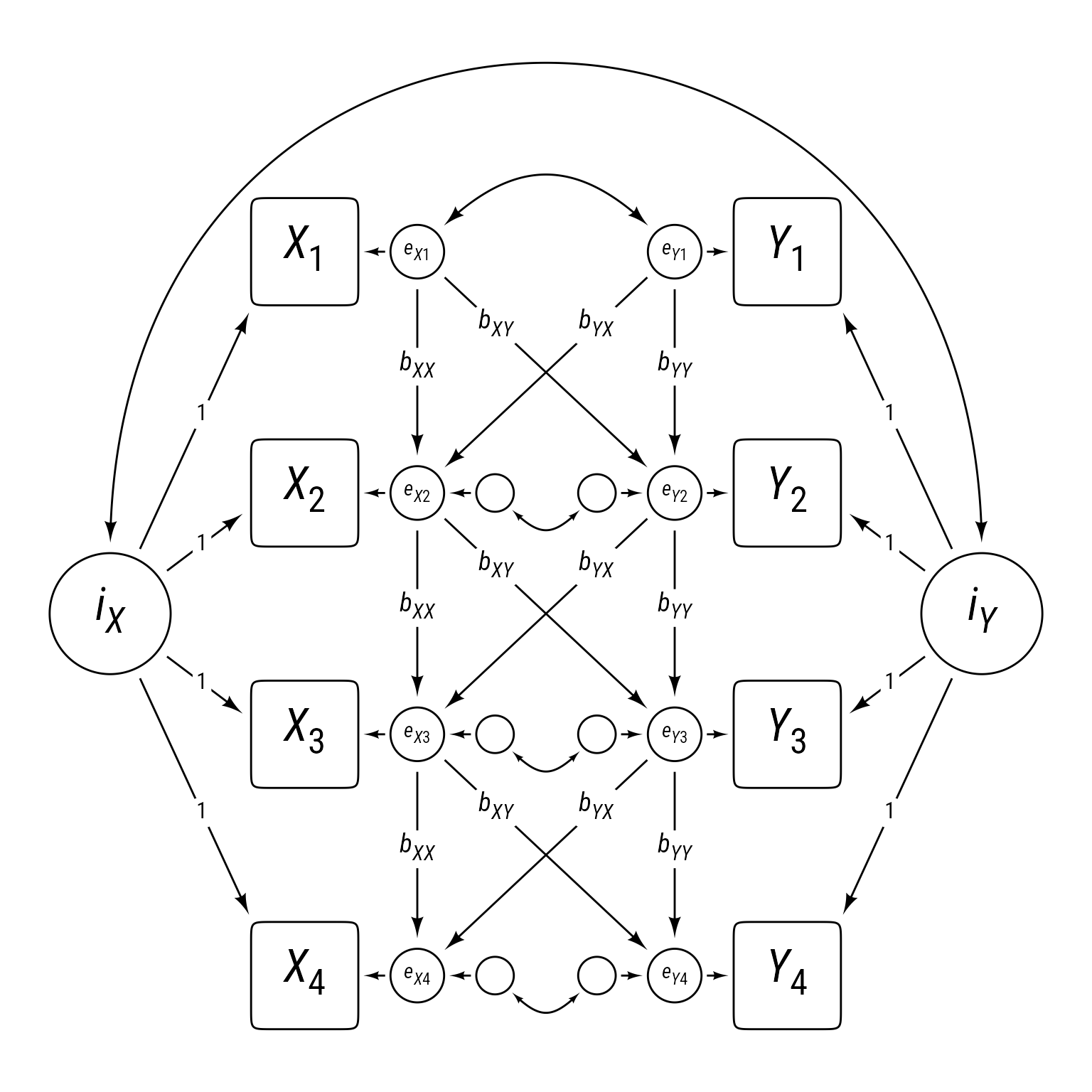

Figure 3: The Cross-Lag Panel Model with Random Intercepts

We need to create latent intercepts for the X and Y series. Here is the syntax we need to define the latent variable I~X:

i_x =~ 1 * x1 + 1 * x2 + 1 * x3 + 1 * x4

If you would rather get that with code instead of typing:

glue("i_x =~ ", 
     glue_collapse(glue("1 * x{1:k}"), 
                   sep = " + "))

i_x =~ 1 * x1 + 1 * x2 + 1 * x3 + 1 * x4

That’s even more typing! I do not want to type that kind of thing for every latent variable.

How about making a custom make_latent function instead?

make_latent <- function(latent, indicator, sep = " + ") {
  glue::glue(
    latent, 
    " =~ ",
    glue::glue_collapse(glue::glue(indicator), sep = sep))
} 

# Less typing!
make_latent(latent = "i_x", indicator = "1 * x{1:k}")

i_x =~ 1 * x1 + 1 * x2 + 1 * x3 + 1 * x4

# Even less typing!
make_latent("i_y", "1 * y{1:k}")

i_y =~ 1 * y1 + 1 * y2 + 1 * y3 + 1 * y4

Structured Residuals

In Figure 3, the residuals for X₂ to X₄ are structured residuals because they have residuals themselves. Technically, structured residuals are not really residuals, but latent variables with loadings of 1.

glue("e_x{1:k} =~ 1 * x{1:k}")

e_x1 =~ 1 * x1
e_x2 =~ 1 * x2
e_x3 =~ 1 * x3
e_x4 =~ 1 * x4

glue("e_y{1:k} =~ 1 * y{1:k}")

e_y1 =~ 1 * y1
e_y2 =~ 1 * y2
e_y3 =~ 1 * y3
e_y4 =~ 1 * y4

To make the structured residuals behave like residuals, we need to set the actual residuals of the observed variables to have 0 variance:

\{r\} #| label:\1 glue("x{1:k} ~~ 0 * x{1:k}") glue("y{1:k} ~~ 0 * y{1:k}")

We also need to label the latent variance and covariance parameters such that the first one is different from the others, which are set equal:

var_ex <- c("tau_ex1", rep("tau_exx", k - 1))
var_ey <- c("tau_ey1", rep("tau_eyy", k - 1))
cov_exy <- c("tau_exy1", rep("tau_exy", k - 1))
glue("e_x{1:k} ~~ {var_ex} * e_x{1:k}")

e_x1 ~~ tau_ex1 * e_x1
e_x2 ~~ tau_exx * e_x2
e_x3 ~~ tau_exx * e_x3
e_x4 ~~ tau_exx * e_x4

glue("e_y{1:k} ~~ {var_ey} * e_y{1:k}")

e_y1 ~~ tau_ey1 * e_y1
e_y2 ~~ tau_eyy * e_y2
e_y3 ~~ tau_eyy * e_y3
e_y4 ~~ tau_eyy * e_y4

glue("e_x{1:k} ~~ {cov_exy} * e_y{1:k}")

e_x1 ~~ tau_exy1 * e_y1
e_x2 ~~ tau_exy * e_y2
e_x3 ~~ tau_exy * e_y3
e_x4 ~~ tau_exy * e_y4

The regression syntax is similar to the CLPM syntax except that the predictors and outcomes are between the structured residuals instead of the observed variables.

glue("e_x{s2k} ~ b_xx * x{s1k1} + b_yx * e_y{s1k1}")

e_x2 ~ b_xx * x1 + b_yx * e_y1
e_x3 ~ b_xx * x2 + b_yx * e_y2
e_x4 ~ b_xx * x3 + b_yx * e_y3

glue("e_y{s2k} ~ b_yy * y{s1k1} + b_xy * e_x{s1k1}")

e_y2 ~ b_yy * y1 + b_xy * e_x1
e_y3 ~ b_yy * y2 + b_xy * e_x2
e_y4 ~ b_yy * y3 + b_xy * e_x3

The latent random intercepts need intercepts (weird but true):

i_x ~ b_ix_0 * 1
i_y ~ b_iy_0 * 1

Finally, the latent random intercepts need variances and a covariance:

i_x ~~ tau_ix * i_x + tau_ixiy * i_y
i_y ~~ tau_iy * i_y

Putting it all together for the RI-CLPM:

# Number of waves
k <- 4
# Sequence from 2 to k
s2k <- seq(2, k)
# Sequence from 1 to k - 1
s1k1 <- seq(1, k - 1)
# Residual variances and covariances
var_ex <- c("tau_ex1", rep("tau_exx", k - 1))
var_ey <- c("tau_ey1", rep("tau_eyy", k - 1))
cov_exy <- c("tau_exy1", rep("tau_exy", k - 1))


m_riclpm <- c("# Latent intercepts",
  make_latent("i_x", "1 * x{1:k}"),
  make_latent("i_y", "1 * y{1:k}"),
  "# Structured Residuals",
  glue("e_x{1:k} =~ 1 * x{1:k}"), 
  glue("e_y{1:k} =~ 1 * y{1:k}"),
  "# Set observed residuals to 0",
  glue("x{1:k} ~~ 0 * x{1:k}"), 
  glue("y{1:k} ~~ 0 * y{1:k}"),
  "# Structured Residual Variances and Covariances",
  glue("e_x{1:k} ~~ {var_ex} * e_x{1:k}"),
  glue("e_y{1:k} ~~ {var_ey} * e_y{1:k}"), 
  glue("e_x{1:k} ~~ {cov_exy} * e_y{1:k}"),
  "# Structured Residual Regressions",
  glue("e_x{s2k} ~ b_xx * e_x{s1k1} + b_yx * e_y{s1k1}"),
  glue("e_y{s2k} ~ b_yy * e_y{s1k1} + b_xy * e_x{s1k1}"),
  "# Observed Intercepts set to 0",
  glue("x{1:k} ~ 0 * 1"), 
  glue("y{1:k} ~ 0 * 1"), 
  "# Random Intercept Intercepts",
  "i_x ~ b_ix_0 * 1",
  "i_y ~ b_iy_0 * 1",
  "# Random Intecept Variances and Covariance",
  "i_x ~~ tau_ix * i_x + tau_ixiy * i_y",
  "i_y ~~ tau_iy * i_y"
  ) %>% 
  glue_collapse("\n") 

m_riclpm

# Latent intercepts
i_x =~ 1 * x1 + 1 * x2 + 1 * x3 + 1 * x4
i_y =~ 1 * y1 + 1 * y2 + 1 * y3 + 1 * y4
# Structured Residuals
e_x1 =~ 1 * x1
e_x2 =~ 1 * x2
e_x3 =~ 1 * x3
e_x4 =~ 1 * x4
e_y1 =~ 1 * y1
e_y2 =~ 1 * y2
e_y3 =~ 1 * y3
e_y4 =~ 1 * y4
# Set observed residuals to 0
x1 ~~ 0 * x1
x2 ~~ 0 * x2
x3 ~~ 0 * x3
x4 ~~ 0 * x4
y1 ~~ 0 * y1
y2 ~~ 0 * y2
y3 ~~ 0 * y3
y4 ~~ 0 * y4
# Structured Residual Variances and Covariances
e_x1 ~~ tau_ex1 * e_x1
e_x2 ~~ tau_exx * e_x2
e_x3 ~~ tau_exx * e_x3
e_x4 ~~ tau_exx * e_x4
e_y1 ~~ tau_ey1 * e_y1
e_y2 ~~ tau_eyy * e_y2
e_y3 ~~ tau_eyy * e_y3
e_y4 ~~ tau_eyy * e_y4
e_x1 ~~ tau_exy1 * e_y1
e_x2 ~~ tau_exy * e_y2
e_x3 ~~ tau_exy * e_y3
e_x4 ~~ tau_exy * e_y4
# Structured Residual Regressions
e_x2 ~ b_xx * e_x1 + b_yx * e_y1
e_x3 ~ b_xx * e_x2 + b_yx * e_y2
e_x4 ~ b_xx * e_x3 + b_yx * e_y3
e_y2 ~ b_yy * e_y1 + b_xy * e_x1
e_y3 ~ b_yy * e_y2 + b_xy * e_x2
e_y4 ~ b_yy * e_y3 + b_xy * e_x3
# Observed Intercepts set to 0
x1 ~ 0 * 1
x2 ~ 0 * 1
x3 ~ 0 * 1
x4 ~ 0 * 1
y1 ~ 0 * 1
y2 ~ 0 * 1
y3 ~ 0 * 1
y4 ~ 0 * 1
# Random Intercept Intercepts
i_x ~ b_ix_0 * 1
i_y ~ b_iy_0 * 1
# Random Intecept Variances and Covariance
i_x ~~ tau_ix * i_x + tau_ixiy * i_y
i_y ~~ tau_iy * i_y

Here we set the parameters for data simulation:

params_riclpm <- c(
  tau_ex1 = 1,
  tau_ey1 = 1,
  tau_exy1 = .4,
  tau_exx = .4,
  tau_eyy = .5,
  tau_exy = .2,
  tau_ix = 0.75,
  tau_iy = 0.75,
  tau_ixiy = .25,
  b_xx = .5,
  b_yy = .4,
  b_xy = .3,
  b_yx = 0,
  b_ix_0 = 0,
  b_iy_0 = 0
) 

d_riclpm <- replace_parameters(model = m_riclpm, 
                   params = params_riclpm) %>% 
  glue_collapse("\n") %>% 
  simulateData(sample.nobs = 1000)

In Figure 4, we can see the correlations among the variables created with the RI-CLPM.

Code

plot_cor(d_riclpm)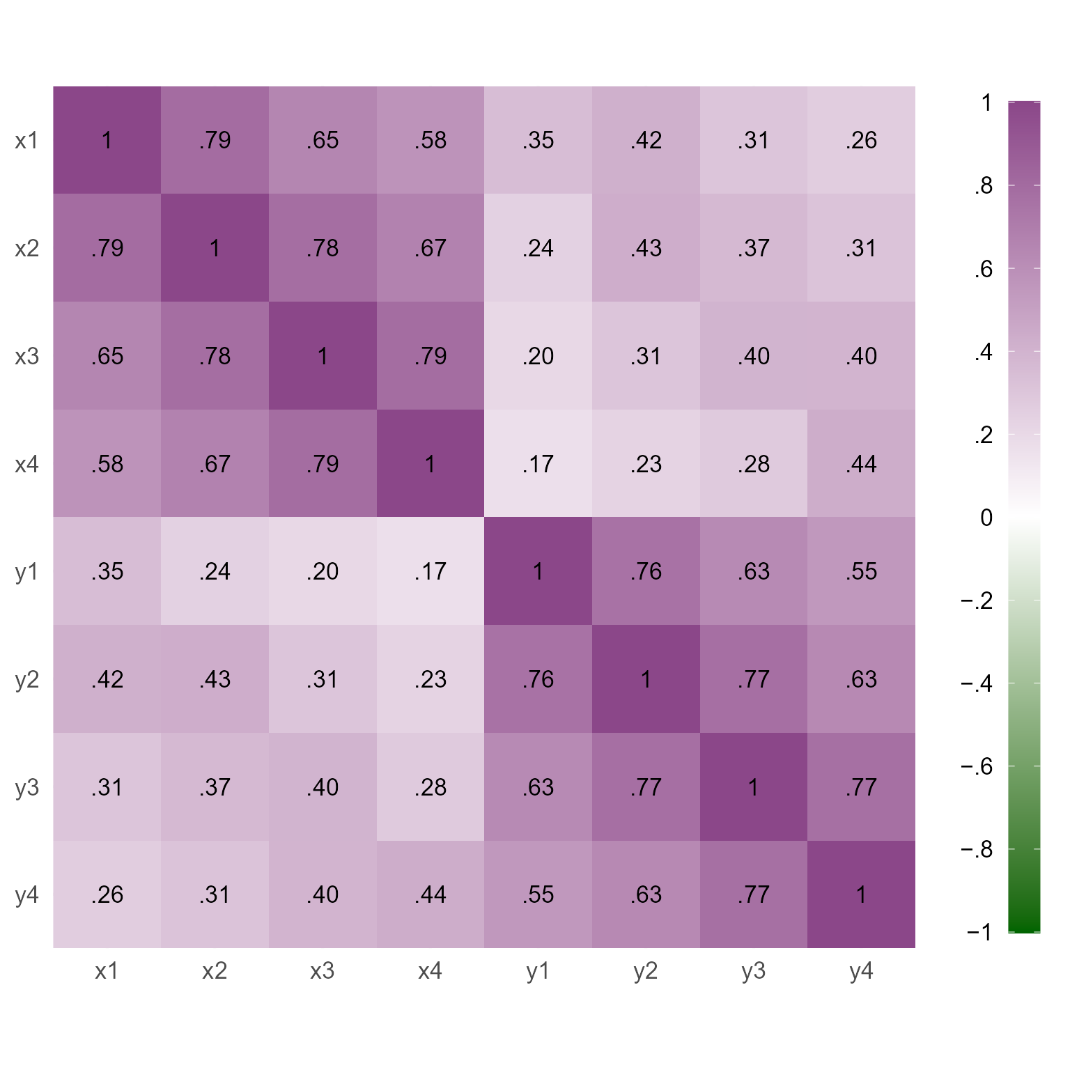

Figure 4: Correlation of X and Y in RI-CLPM

In Figure 5, we see that the RI-CLPM creates data that stays at the same overall level across time. There is no growth.

Code

library(gganimate)
d_riclpm %>%
  tibble::rowid_to_column("id") %>%
  pivot_longer(-id) %>%
  mutate(v = str_sub(name, 1, 1),
         time = str_sub(name, 2, 2) %>% as.integer()) %>%
  select(-name) %>%
  pivot_wider(names_from = v) %>%
  mutate(id = fct_reorder(factor(id), x, .fun = mean)) %>%
  ggplot(aes(x, y)) +
  geom_point(aes(color = id), pch = 16) +
  transition_states(time, .75, 3) +
  ease_aes('cubic-in-out') +
  shadow_wake(wake_length = 0.15) +
  theme_minimal(base_size = 24, base_family = "Roboto Condensed") +
  theme(legend.position = "none",
        axis.title.y = element_text(
          angle = 0,
          hjust = .5,
          vjust = .5
        )) +
  scale_color_viridis_d() +
  labs(title = 'Time {closest_state}', x = 'X', y = 'Y')

Figure 5: Changes in X and Y over Time in RI-CLPM

Figure 6 show the distributions over time in the RI-CLPM. It is evident that the model does not allow for change over time (by design). If we expect growth, we need a model that allows for growth.

Code

d_riclpm %>%
  tibble::rowid_to_column("id") %>%
  pivot_longer(-id) %>%
  mutate(v = str_sub(name, 1, 1),
         time = str_sub(name, 2, 2) %>% as.integer() %>% factor()) %>%
  mutate(id = fct_reorder(factor(id), value, .fun = mean)) %>%
  select(-name) %>%
  
  ggplot(aes(time, value)) +
  geom_violin(color = NA, fill = "gray95") +
  geom_line(aes(group = id, color = id), linewidth = .2, alpha = .1) +
  facet_grid(cols = vars(v)) +
  scale_color_viridis_d() +
  theme_light(base_size = 24, base_family = "Roboto Condensed") +
  theme(legend.position = "none",
        axis.title.y = element_text(
          angle = 0,
          hjust = .5,
          vjust = .5
        )) +
  labs(y = NULL, x = "Time")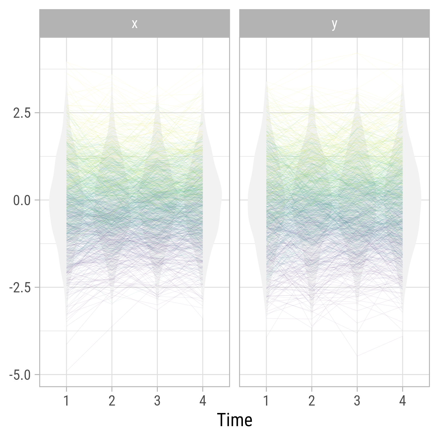

Figure 6: Distribution of X and Y over Time in RI-CLPM

If we did not know how the data were generated, we could evaluate the model with the RI-CLPM.

sem(model = m_riclpm, data = d_riclpm, auto.cov.lv.x = F) %>% 
  model_parameters(component = "all")

# Loading

Link       | Coefficient |   SE |       95% CI |      p
-------------------------------------------------------
i_x =~ x1  |        1.00 | 0.00 | [1.00, 1.00] | < .001
i_x =~ x2  |        1.00 | 0.00 | [1.00, 1.00] | < .001
i_x =~ x3  |        1.00 | 0.00 | [1.00, 1.00] | < .001
i_x =~ x4  |        1.00 | 0.00 | [1.00, 1.00] | < .001
i_y =~ y1  |        1.00 | 0.00 | [1.00, 1.00] | < .001
i_y =~ y2  |        1.00 | 0.00 | [1.00, 1.00] | < .001
i_y =~ y3  |        1.00 | 0.00 | [1.00, 1.00] | < .001
i_y =~ y4  |        1.00 | 0.00 | [1.00, 1.00] | < .001
e_x1 =~ x1 |        1.00 | 0.00 | [1.00, 1.00] | < .001
e_x2 =~ x2 |        1.00 | 0.00 | [1.00, 1.00] | < .001
e_x3 =~ x3 |        1.00 | 0.00 | [1.00, 1.00] | < .001
e_x4 =~ x4 |        1.00 | 0.00 | [1.00, 1.00] | < .001
e_y1 =~ y1 |        1.00 | 0.00 | [1.00, 1.00] | < .001
e_y2 =~ y2 |        1.00 | 0.00 | [1.00, 1.00] | < .001
e_y3 =~ y3 |        1.00 | 0.00 | [1.00, 1.00] | < .001
e_y4 =~ y4 |        1.00 | 0.00 | [1.00, 1.00] | < .001

# Variance

Link                   | Coefficient |   SE |       95% CI |     z |      p
---------------------------------------------------------------------------
x1 ~~ x1               |        0.00 | 0.00 | [0.00, 0.00] |       | < .001
x2 ~~ x2               |        0.00 | 0.00 | [0.00, 0.00] |       | < .001
x3 ~~ x3               |        0.00 | 0.00 | [0.00, 0.00] |       | < .001
x4 ~~ x4               |        0.00 | 0.00 | [0.00, 0.00] |       | < .001
y1 ~~ y1               |        0.00 | 0.00 | [0.00, 0.00] |       | < .001
y2 ~~ y2               |        0.00 | 0.00 | [0.00, 0.00] |       | < .001
y3 ~~ y3               |        0.00 | 0.00 | [0.00, 0.00] |       | < .001
y4 ~~ y4               |        0.00 | 0.00 | [0.00, 0.00] |       | < .001
e_x1 ~~ e_x1 (tau_ex1) |        0.96 | 0.07 | [0.83, 1.10] | 13.93 | < .001
e_x2 ~~ e_x2 (tau_exx) |        0.40 | 0.02 | [0.37, 0.44] | 25.79 | < .001
e_x3 ~~ e_x3 (tau_exx) |        0.40 | 0.02 | [0.37, 0.44] | 25.79 | < .001
e_x4 ~~ e_x4 (tau_exx) |        0.40 | 0.02 | [0.37, 0.44] | 25.79 | < .001
e_y1 ~~ e_y1 (tau_ey1) |        0.95 | 0.07 | [0.80, 1.09] | 12.72 | < .001
e_y2 ~~ e_y2 (tau_eyy) |        0.50 | 0.02 | [0.47, 0.54] | 26.42 | < .001
e_y3 ~~ e_y3 (tau_eyy) |        0.50 | 0.02 | [0.47, 0.54] | 26.42 | < .001
e_y4 ~~ e_y4 (tau_eyy) |        0.50 | 0.02 | [0.47, 0.54] | 26.42 | < .001
i_x ~~ i_x (tau_ix)    |        0.71 | 0.06 | [0.59, 0.83] | 11.58 | < .001
i_y ~~ i_y (tau_iy)    |        0.76 | 0.08 | [0.60, 0.91] |  9.82 | < .001

# Correlation

Link                    | Coefficient |   SE |       95% CI |     z |      p
----------------------------------------------------------------------------
e_x1 ~~ e_y1 (tau_exy1) |        0.40 | 0.06 | [0.29, 0.52] |  6.88 | < .001
e_x2 ~~ e_y2 (tau_exy)  |        0.20 | 0.01 | [0.18, 0.23] | 15.55 | < .001
e_x3 ~~ e_y3 (tau_exy)  |        0.20 | 0.01 | [0.18, 0.23] | 15.55 | < .001
e_x4 ~~ e_y4 (tau_exy)  |        0.20 | 0.01 | [0.18, 0.23] | 15.55 | < .001
i_x ~~ i_y (tau_ixiy)   |        0.20 | 0.06 | [0.09, 0.31] |  3.58 | < .001

# Regression

Link               | Coefficient |   SE |        95% CI |     z |      p
------------------------------------------------------------------------
e_x2 ~ e_x1 (b_xx) |        0.50 | 0.03 | [ 0.44, 0.57] | 15.26 | < .001
e_x2 ~ e_y1 (b_yx) |    3.02e-03 | 0.03 | [-0.05, 0.05] |  0.11 | 0.909 
e_x3 ~ e_x2 (b_xx) |        0.50 | 0.03 | [ 0.44, 0.57] | 15.26 | < .001
e_x3 ~ e_y2 (b_yx) |    3.02e-03 | 0.03 | [-0.05, 0.05] |  0.11 | 0.909 
e_x4 ~ e_x3 (b_xx) |        0.50 | 0.03 | [ 0.44, 0.57] | 15.26 | < .001
e_x4 ~ e_y3 (b_yx) |    3.02e-03 | 0.03 | [-0.05, 0.05] |  0.11 | 0.909 
e_y2 ~ e_y1 (b_yy) |        0.39 | 0.04 | [ 0.32, 0.46] | 11.09 | < .001
e_y2 ~ e_x1 (b_xy) |        0.33 | 0.03 | [ 0.27, 0.39] | 11.26 | < .001
e_y3 ~ e_y2 (b_yy) |        0.39 | 0.04 | [ 0.32, 0.46] | 11.09 | < .001
e_y3 ~ e_x2 (b_xy) |        0.33 | 0.03 | [ 0.27, 0.39] | 11.26 | < .001
e_y4 ~ e_y3 (b_yy) |        0.39 | 0.04 | [ 0.32, 0.46] | 11.09 | < .001
e_y4 ~ e_x3 (b_xy) |        0.33 | 0.03 | [ 0.27, 0.39] | 11.26 | < .001

# Mean

Link             | Coefficient |   SE |        95% CI |     z |      p
----------------------------------------------------------------------
x1 ~1            |        0.00 | 0.00 | [ 0.00, 0.00] |       | < .001
x2 ~1            |        0.00 | 0.00 | [ 0.00, 0.00] |       | < .001
x3 ~1            |        0.00 | 0.00 | [ 0.00, 0.00] |       | < .001
x4 ~1            |        0.00 | 0.00 | [ 0.00, 0.00] |       | < .001
y1 ~1            |        0.00 | 0.00 | [ 0.00, 0.00] |       | < .001
y2 ~1            |        0.00 | 0.00 | [ 0.00, 0.00] |       | < .001
y3 ~1            |        0.00 | 0.00 | [ 0.00, 0.00] |       | < .001
y4 ~1            |        0.00 | 0.00 | [ 0.00, 0.00] |       | < .001
i_x ~1  (b_ix_0) |       -0.02 | 0.03 | [-0.08, 0.04] | -0.60 | 0.547 
i_y ~1  (b_iy_0) |       -0.01 | 0.03 | [-0.08, 0.06] | -0.37 | 0.713 
e_x1 ~1          |        0.00 | 0.00 | [ 0.00, 0.00] |       | < .001
e_x2 ~1          |        0.00 | 0.00 | [ 0.00, 0.00] |       | < .001
e_x3 ~1          |        0.00 | 0.00 | [ 0.00, 0.00] |       | < .001
e_x4 ~1          |        0.00 | 0.00 | [ 0.00, 0.00] |       | < .001
e_y1 ~1          |        0.00 | 0.00 | [ 0.00, 0.00] |       | < .001
e_y2 ~1          |        0.00 | 0.00 | [ 0.00, 0.00] |       | < .001
e_y3 ~1          |        0.00 | 0.00 | [ 0.00, 0.00] |       | < .001
e_y4 ~1          |        0.00 | 0.00 | [ 0.00, 0.00] |       | < .001

Latent Growth With Structured Residuals

Here we combine bivariate latent growth models with the cross-lagged panel model (Curran et al., 2014).

Curran, P. J., Howard, A. L., Bainter, S. A., Lane, S. T., & McGinley, J. S. (2014). The separation of between-person and within-person components of individual change over time: A latent curve model with structured residuals. Journal of Consulting and Clinical Psychology, 82(5), 879–894. https://doi.org/10.1037/a0035297

Code

ggdiagram(font_family = my_font, font_size = 24) +
  {x <- my_observed() %>%
    ob_array(k,
             sep = 2.5,
             where = "south",
             label = paste0("*X*~" , 1:k, "~"))} +
  {y <- my_observed(label = paste0("*Y*~" ,1:k, "~")) %>%  
    place(x, "right", sep = 6)} +
  {e_x <- my_error(radius = .5) %>% place(x, "right", sep = .5)} +
  {e_y <- my_error(radius = .5) %>% place(y, "left", sep = .5)} +
  {ee_x <- my_error() %>% place(e_x[-1], "right", sep = .5)} +
  {ee_y <- my_error() %>% place(e_y[-1], "left", sep = .5)} +
  {lxx <- my_connect(e_x[-k], e_x[-1])} +
  ob_label("*b~XX~*", lxx@midpoint(.47), size = 14) +
  {lxy <- my_connect(e_x[-k], e_y[-1])} +
  ob_label("*b~XY~*", lxy@midpoint(.27), size = 14) +
  {lyx <- my_connect(e_y[-k], e_x[-1])} +
  ob_label("*b~YX~*", lyx@midpoint(.27), size = 14) +
  {lyy <- my_connect(e_y[-k], e_y[-1])} + 
  ob_label("*b~YY~*", lyy@midpoint(.47), size = 14) +
  my_connect2(e_x, x) + 
  my_connect2(e_y, y) +
  my_connect2(ee_x, e_x[-1]) +
  my_connect2(ee_y, e_y[-1]) +
  ob_covariance(e_x[1], e_y[1]) + 
  ob_covariance(ee_y, ee_x, 
                resect = 1,
                length_head = 4, 
                length_fins = 4, 
                looseness = 1.3) +
  {ix <- ob_circle(label = "*i*~*X*~", radius = sqrt(4 / pi)) %>% 
    place(x[2]@bounding_box@point_at("left"), "left", sep = 3)} +
  {iy <- ob_circle(label = "*i*~*Y*~", radius = sqrt(4 / pi)) %>% 
    place(y[2]@bounding_box@point_at("right"), "right", sep = 3)} + 
  {sx <- ob_circle(label = "*s*~*X*~", radius = sqrt(4 / pi)) %>% 
    place(x[3]@bounding_box@point_at("left"), "left", sep = 3)} +
  {sy <- ob_circle(label = "*s*~*Y*~", radius = sqrt(4 / pi)) %>% 
    place(y[3]@bounding_box@point_at("right"), "right", sep = 3)} + 
  {lx <- my_connect(ix, x@point_at(degree(175)))} +
  {ly <- my_connect(iy, y@point_at(degree(5)))} + 
  ob_label("1",
           center = lx@line@point_at_x(lx[2]@midpoint(.66)@x),
           size = 12) +
  ob_label("1",
           center = ly@line@point_at_x(ly[2]@midpoint(.66)@x),
           size = 12) + 
  {lsx <- my_connect(sx, x@point_at(degree(185)))} +
  {lsy <- my_connect(sy, y@point_at(degree(-5)))} + 
  ob_label(0:3,
           center = lsx@line@point_at_x(lsx[3]@midpoint(.66)@x),
           size = 12) +
  ob_label(0:3,
           center = lsy@line@point_at_x(lsy[3]@midpoint(.66)@x),
           size = 12) +
  ob_covariance(ix@point_at(degree(80)), 
                iy@point_at(degree(100)), 
                looseness = 1.1, 
                bend = 40) +
  ob_covariance(ix@point_at(degree(95)), 
                sy@point_at(degree(55)), 
                looseness = 1.5, 
                bend = 60) +
  ob_covariance(sy@point_at(degree(260)), 
                sx@point_at(degree(280)), 
                looseness = 1.1, 
                bend = 40) +
  ob_covariance(sy@point_at(degree(285)), 
                ix@point_at(degree(235)), 
                looseness = 1.5, 
                bend = 60) +
  ob_covariance(iy@point_at(degree(-70)), 
                sy@point_at(degree(70)), 
                bend = degree(-20)) +
  ob_covariance(sx@point_at(degree(110)), 
                ix@point_at(degree(-110)), 
                bend = degree(-20))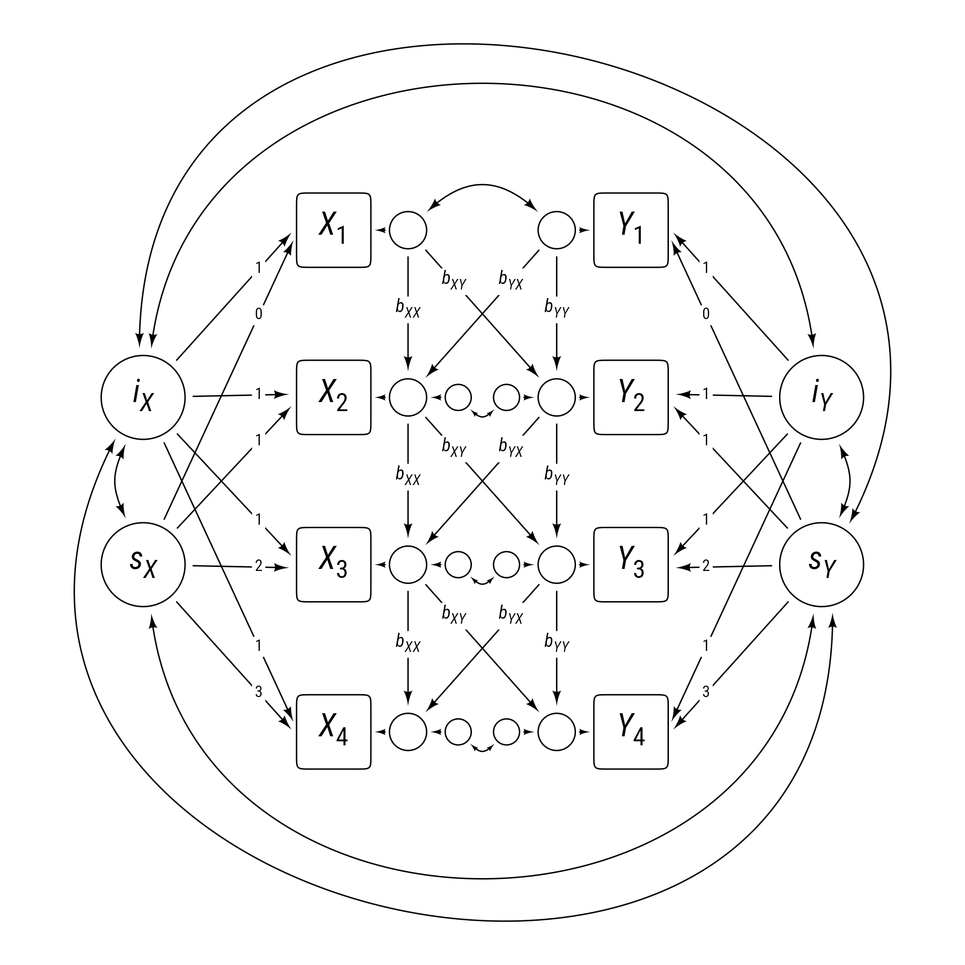

Figure 7: The Latent Growth Model with Structured Residuals

The Latent Growth with Structured Residuals Model is exactly the same as the RI-CLPM but it adds growth in the form of random latent slopes, s_X and s_Y and the covariances among the random latent slopes and random latent intercepts.

# Number of waves
k <- 4
# Sequence from 2 to k
s2k <- seq(2, k)
# Sequence from 1 to k - 1
s1k1 <- seq(1, k - 1)
# Residual variances and covariances
var_ex <- c("tau_ex1", rep("tau_exx", k - 1))
var_ey <- c("tau_ey1", rep("tau_eyy", k - 1))
cov_exy <- c("tau_exy1", rep("tau_exy", k - 1))


m_lgsr <- c("# Random Latent Intercepts",
  make_latent("i_x", "1 * x{1:k}"),
  make_latent("i_y", "1 * y{1:k}"),
  "# Random Latent Slopes",
  make_latent("s_x", "{seq(0,k-1)} * x{1:k}"),
  make_latent("s_y", "{seq(0,k-1)} * y{1:k}"),
  "# Structured Residuals",
  glue("e_x{1:k} =~ 1 * x{1:k}"), 
  glue("e_y{1:k} =~ 1 * y{1:k}"),
  "# Set observed residuals to 0",
  glue("x{1:k} ~~ 0 * x{1:k}"), 
  glue("y{1:k} ~~ 0 * y{1:k}"),
  "# Structured Residual Variances and Covariances",
  glue("e_x{1:k} ~~ {var_ex} * e_x{1:k}"),
  glue("e_y{1:k} ~~ {var_ey} * e_y{1:k}"), 
  glue("e_x{1:k} ~~ {cov_exy} * e_y{1:k}"),
  "# Structured Residual Regressions",
  glue("e_x{s2k} ~ b_xx * x{s1k1} + b_yx * e_y{s1k1}"),
  glue("e_y{s2k} ~ b_yy * y{s1k1} + b_xy * e_x{s1k1}"),
  "# Observed Intercepts",
  glue("x{1:k} ~ 0 * 1"), 
  glue("y{1:k} ~ 0 * 1"), 
  "# Random Intercept Intercepts",
  "i_x ~ b_ix_0 * 1",
  "i_y ~ b_iy_0 * 1",
  "# Random Slope Intercepts",
  "s_x ~ b_sx_0 * 1",
  "s_y ~ b_sy_0 * 1",
  "# Random Intecept Variances and Covariance",
  "i_x ~~ tau_ix * i_x + tau_ixiy * i_y + tau_ixsx * s_x + tau_ixsy * s_y",
  "i_y ~~ tau_iy * i_y + tau_iysx * s_x + tau_iysy * s_y", 
  "s_x ~~ tau_sx * s_x + tau_sxsy * s_y",
  "s_y ~~ tau_sy * s_y"
  ) %>% 
  glue_collapse("\n") 

m_lgsr

# Random Latent Intercepts
i_x =~ 1 * x1 + 1 * x2 + 1 * x3 + 1 * x4
i_y =~ 1 * y1 + 1 * y2 + 1 * y3 + 1 * y4
# Random Latent Slopes
s_x =~ 0 * x1 + 1 * x2 + 2 * x3 + 3 * x4
s_y =~ 0 * y1 + 1 * y2 + 2 * y3 + 3 * y4
# Structured Residuals
e_x1 =~ 1 * x1
e_x2 =~ 1 * x2
e_x3 =~ 1 * x3
e_x4 =~ 1 * x4
e_y1 =~ 1 * y1
e_y2 =~ 1 * y2
e_y3 =~ 1 * y3
e_y4 =~ 1 * y4
# Set observed residuals to 0
x1 ~~ 0 * x1
x2 ~~ 0 * x2
x3 ~~ 0 * x3
x4 ~~ 0 * x4
y1 ~~ 0 * y1
y2 ~~ 0 * y2
y3 ~~ 0 * y3
y4 ~~ 0 * y4
# Structured Residual Variances and Covariances
e_x1 ~~ tau_ex1 * e_x1
e_x2 ~~ tau_exx * e_x2
e_x3 ~~ tau_exx * e_x3
e_x4 ~~ tau_exx * e_x4
e_y1 ~~ tau_ey1 * e_y1
e_y2 ~~ tau_eyy * e_y2
e_y3 ~~ tau_eyy * e_y3
e_y4 ~~ tau_eyy * e_y4
e_x1 ~~ tau_exy1 * e_y1
e_x2 ~~ tau_exy * e_y2
e_x3 ~~ tau_exy * e_y3
e_x4 ~~ tau_exy * e_y4
# Structured Residual Regressions
e_x2 ~ b_xx * x1 + b_yx * e_y1
e_x3 ~ b_xx * x2 + b_yx * e_y2
e_x4 ~ b_xx * x3 + b_yx * e_y3
e_y2 ~ b_yy * y1 + b_xy * e_x1
e_y3 ~ b_yy * y2 + b_xy * e_x2
e_y4 ~ b_yy * y3 + b_xy * e_x3
# Observed Intercepts
x1 ~ 0 * 1
x2 ~ 0 * 1
x3 ~ 0 * 1
x4 ~ 0 * 1
y1 ~ 0 * 1
y2 ~ 0 * 1
y3 ~ 0 * 1
y4 ~ 0 * 1
# Random Intercept Intercepts
i_x ~ b_ix_0 * 1
i_y ~ b_iy_0 * 1
# Random Slope Intercepts
s_x ~ b_sx_0 * 1
s_y ~ b_sy_0 * 1
# Random Intecept Variances and Covariance
i_x ~~ tau_ix * i_x + tau_ixiy * i_y + tau_ixsx * s_x + tau_ixsy * s_y
i_y ~~ tau_iy * i_y + tau_iysx * s_x + tau_iysy * s_y
s_x ~~ tau_sx * s_x + tau_sxsy * s_y
s_y ~~ tau_sy * s_y

Let’s make the random slope for X be negative (b_sx_0 = -.25), on average, and the random slope for Y be positive (b_sy_0 = .5), on average.

params_lgsr <- c(
  tau_ex1 = 1,
  tau_ey1 = 1,
  tau_exy1 = .4,
  tau_exx = .4,
  tau_eyy = .5,
  tau_exy = .2,
  tau_ix = 0.5,
  tau_iy = 0.6,
  tau_sx = 0.1,
  tau_sy = 0.2,
  tau_ixiy = .3,
  tau_ixsy = 0,
  tau_ixsx = .03,
  tau_iysx = 0,
  tau_iysy = -.02,
  tau_sxsy = 0.01,
  b_xx = .4,
  b_yy = .3,
  b_xy = .1,
  b_yx = 0,
  b_ix_0 = 0,
  b_iy_0 = 0,
  b_sx_0 = -.25,
  b_sy_0 = .5
) 

d_lgsr <- replace_parameters(model = m_lgsr, 
                   params = params_lgsr) %>% 
  glue_collapse("\n") %>% 
  simulateData(sample.nobs = 1000)

fit_lgsr <- sem(model = m_lgsr, data = d_lgsr, auto.cov.lv.x = F)

All the variables are still positively correlated:

Code

plot_cor(d_lgsr)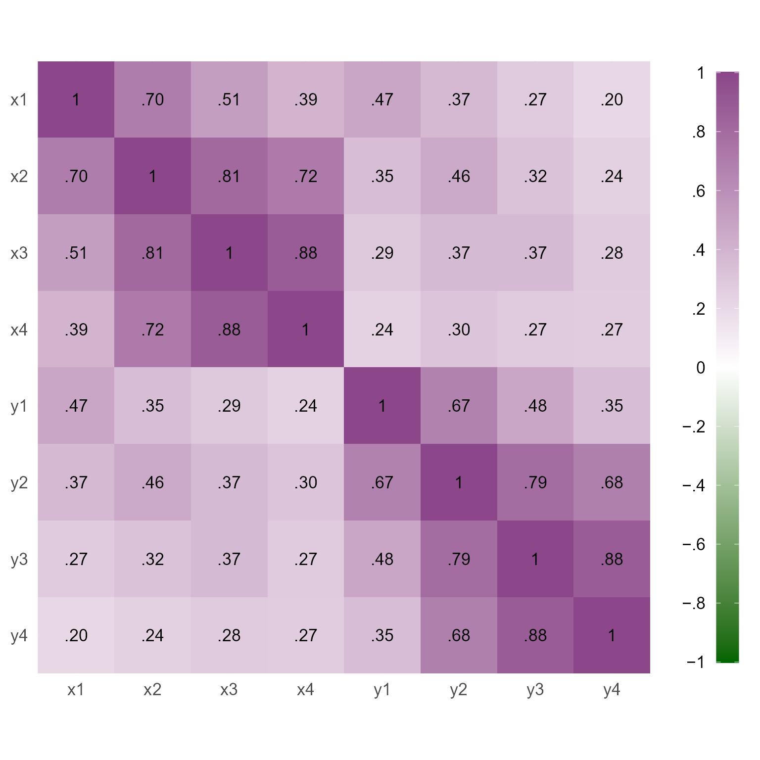

Figure 8: Correlation of X and Y in LGSR Model

But, over time, X decreases, and Y increases.

Code

library(gganimate)
d_lgsr %>% 
  tibble::rowid_to_column("id") %>% 
  pivot_longer(-id) %>% 
  mutate(v = str_sub(name, 1,1),
         time = str_sub(name, 2,2) %>% as.integer()) %>% 
  select(-name) %>% 
  pivot_wider(names_from = v) %>% 
  mutate(id = fct_reorder(factor(id), x, .fun = mean)) %>% 
  ggplot(aes(x,y)) + 
  geom_point(aes(color = id), pch = 16) + 
  transition_states(time, .75, 3) +
  ease_aes('cubic-in-out') +
  shadow_wake(wake_length = 0.15) +
  theme_minimal(base_size = 24, base_family = "Roboto Condensed") +
  theme(legend.position = "none", axis.title.y = element_text(angle = 0, hjust = .5, vjust=.5)) +
  scale_color_viridis_d() +
  labs(title = 'Time {closest_state}', x = 'X', y = 'Y')

Figure 9: Changes in X and Y over Time in LGSR Model

See the slopes for the two variables:

Code

d_lgsr %>% 
  tibble::rowid_to_column("id") %>% 
  pivot_longer(-id) %>% 
  mutate(v = str_sub(name, 1,1),
         time = str_sub(name, 2,2) %>% as.integer() %>% factor()) %>% 
  mutate(id = fct_reorder(factor(id), value, .fun = mean)) %>% 
  select(-name) %>%
  
  ggplot(aes(time, value)) + 
  geom_violin(color = NA, fill = "gray95") + 
  geom_line(aes(group = id, color = id), size = .2, alpha = .1) + 
  geom_smooth(aes(x = as.integer(time)), method = "lm") +
  facet_grid(cols = vars(v)) + 
  scale_color_viridis_d() +
  theme_light(base_size = 24, base_family = "Roboto Condensed") +
  theme(legend.position = "none", axis.title.y = element_text(angle = 0, hjust = .5, vjust = .5)) + 
  labs(y = NULL, x = "Time")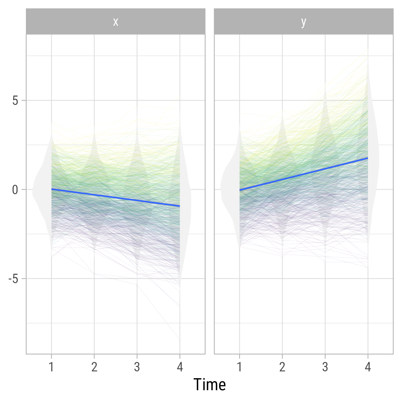

Figure 10: Distribution of X and Y over Time in LGSR Model

Testing the model

sem(model = m_lgsr, data = d_lgsr, auto.cov.lv.x = F) %>% 
  model_parameters(component = "all")

# Loading

Link       | Coefficient |   SE |       95% CI |      p
-------------------------------------------------------
i_x =~ x1  |        1.00 | 0.00 | [1.00, 1.00] | < .001
i_x =~ x2  |        1.00 | 0.00 | [1.00, 1.00] | < .001
i_x =~ x3  |        1.00 | 0.00 | [1.00, 1.00] | < .001
i_x =~ x4  |        1.00 | 0.00 | [1.00, 1.00] | < .001
i_y =~ y1  |        1.00 | 0.00 | [1.00, 1.00] | < .001
i_y =~ y2  |        1.00 | 0.00 | [1.00, 1.00] | < .001
i_y =~ y3  |        1.00 | 0.00 | [1.00, 1.00] | < .001
i_y =~ y4  |        1.00 | 0.00 | [1.00, 1.00] | < .001
s_x =~ x1  |        0.00 | 0.00 | [0.00, 0.00] | < .001
s_x =~ x2  |        1.00 | 0.00 | [1.00, 1.00] | < .001
s_x =~ x3  |        2.00 | 0.00 | [2.00, 2.00] | < .001
s_x =~ x4  |        3.00 | 0.00 | [3.00, 3.00] | < .001
s_y =~ y1  |        0.00 | 0.00 | [0.00, 0.00] | < .001
s_y =~ y2  |        1.00 | 0.00 | [1.00, 1.00] | < .001
s_y =~ y3  |        2.00 | 0.00 | [2.00, 2.00] | < .001
s_y =~ y4  |        3.00 | 0.00 | [3.00, 3.00] | < .001
e_x1 =~ x1 |        1.00 | 0.00 | [1.00, 1.00] | < .001
e_x2 =~ x2 |        1.00 | 0.00 | [1.00, 1.00] | < .001
e_x3 =~ x3 |        1.00 | 0.00 | [1.00, 1.00] | < .001
e_x4 =~ x4 |        1.00 | 0.00 | [1.00, 1.00] | < .001
e_y1 =~ y1 |        1.00 | 0.00 | [1.00, 1.00] | < .001
e_y2 =~ y2 |        1.00 | 0.00 | [1.00, 1.00] | < .001
e_y3 =~ y3 |        1.00 | 0.00 | [1.00, 1.00] | < .001
e_y4 =~ y4 |        1.00 | 0.00 | [1.00, 1.00] | < .001

# Variance

Link                   | Coefficient |   SE |       95% CI |     z |      p
---------------------------------------------------------------------------
x1 ~~ x1               |        0.00 | 0.00 | [0.00, 0.00] |       | < .001
x2 ~~ x2               |        0.00 | 0.00 | [0.00, 0.00] |       | < .001
x3 ~~ x3               |        0.00 | 0.00 | [0.00, 0.00] |       | < .001
x4 ~~ x4               |        0.00 | 0.00 | [0.00, 0.00] |       | < .001
y1 ~~ y1               |        0.00 | 0.00 | [0.00, 0.00] |       | < .001
y2 ~~ y2               |        0.00 | 0.00 | [0.00, 0.00] |       | < .001
y3 ~~ y3               |        0.00 | 0.00 | [0.00, 0.00] |       | < .001
y4 ~~ y4               |        0.00 | 0.00 | [0.00, 0.00] |       | < .001
e_x1 ~~ e_x1 (tau_ex1) |        0.71 | 0.10 | [0.52, 0.90] |  7.39 | < .001
e_x2 ~~ e_x2 (tau_exx) |        0.33 | 0.02 | [0.28, 0.37] | 14.32 | < .001
e_x3 ~~ e_x3 (tau_exx) |        0.33 | 0.02 | [0.28, 0.37] | 14.32 | < .001
e_x4 ~~ e_x4 (tau_exx) |        0.33 | 0.02 | [0.28, 0.37] | 14.32 | < .001
e_y1 ~~ e_y1 (tau_ey1) |        0.91 | 0.11 | [0.69, 1.13] |  8.09 | < .001
e_y2 ~~ e_y2 (tau_eyy) |        0.46 | 0.03 | [0.39, 0.52] | 14.23 | < .001
e_y3 ~~ e_y3 (tau_eyy) |        0.46 | 0.03 | [0.39, 0.52] | 14.23 | < .001
e_y4 ~~ e_y4 (tau_eyy) |        0.46 | 0.03 | [0.39, 0.52] | 14.23 | < .001
i_x ~~ i_x (tau_ix)    |        0.81 | 0.11 | [0.60, 1.02] |  7.54 | < .001
i_y ~~ i_y (tau_iy)    |        0.68 | 0.11 | [0.45, 0.90] |  5.90 | < .001
s_x ~~ s_x (tau_sx)    |        0.18 | 0.03 | [0.13, 0.24] |  6.74 | < .001
s_y ~~ s_y (tau_sy)    |        0.20 | 0.03 | [0.13, 0.26] |  6.12 | < .001

# Correlation

Link                    | Coefficient |   SE |        95% CI |     z |      p
-----------------------------------------------------------------------------
e_x1 ~~ e_y1 (tau_exy1) |        0.34 | 0.09 | [ 0.16, 0.51] |  3.84 | < .001
e_x2 ~~ e_y2 (tau_exy)  |        0.16 | 0.03 | [ 0.09, 0.22] |  4.60 | < .001
e_x3 ~~ e_y3 (tau_exy)  |        0.16 | 0.03 | [ 0.09, 0.22] |  4.60 | < .001
e_x4 ~~ e_y4 (tau_exy)  |        0.16 | 0.03 | [ 0.09, 0.22] |  4.60 | < .001
i_x ~~ i_y (tau_ixiy)   |        0.39 | 0.09 | [ 0.22, 0.56] |  4.47 | < .001
i_x ~~ s_x (tau_ixsx)   |       -0.03 | 0.02 | [-0.08, 0.02] | -1.17 | 0.243 
i_x ~~ s_y (tau_ixsy)   |       -0.02 | 0.03 | [-0.08, 0.04] | -0.69 | 0.491 
i_y ~~ s_x (tau_iysx)   |        0.02 | 0.03 | [-0.03, 0.07] |  0.79 | 0.427 
i_y ~~ s_y (tau_iysy)   |       -0.01 | 0.03 | [-0.07, 0.04] | -0.39 | 0.699 
s_x ~~ s_y (tau_sxsy)   |        0.01 | 0.02 | [-0.02, 0.05] |  0.73 | 0.465 

# Regression

Link               | Coefficient |   SE |        95% CI |    z |      p
-----------------------------------------------------------------------
e_x2 ~ x1 (b_xx)   |        0.22 | 0.05 | [ 0.13, 0.32] | 4.55 | < .001
e_x2 ~ e_y1 (b_yx) |    5.27e-03 | 0.06 | [-0.11, 0.12] | 0.09 | 0.929 
e_x3 ~ x2 (b_xx)   |        0.22 | 0.05 | [ 0.13, 0.32] | 4.55 | < .001
e_x3 ~ e_y2 (b_yx) |    5.27e-03 | 0.06 | [-0.11, 0.12] | 0.09 | 0.929 
e_x4 ~ x3 (b_xx)   |        0.22 | 0.05 | [ 0.13, 0.32] | 4.55 | < .001
e_x4 ~ e_y3 (b_yx) |    5.27e-03 | 0.06 | [-0.11, 0.12] | 0.09 | 0.929 
e_y2 ~ y1 (b_yy)   |        0.32 | 0.05 | [ 0.22, 0.42] | 6.28 | < .001
e_y2 ~ e_x1 (b_xy) |        0.02 | 0.08 | [-0.13, 0.17] | 0.24 | 0.807 
e_y3 ~ y2 (b_yy)   |        0.32 | 0.05 | [ 0.22, 0.42] | 6.28 | < .001
e_y3 ~ e_x2 (b_xy) |        0.02 | 0.08 | [-0.13, 0.17] | 0.24 | 0.807 
e_y4 ~ y3 (b_yy)   |        0.32 | 0.05 | [ 0.22, 0.42] | 6.28 | < .001
e_y4 ~ e_x3 (b_xy) |        0.02 | 0.08 | [-0.13, 0.17] | 0.24 | 0.807 

# Mean

Link             | Coefficient |   SE |         95% CI |      z |      p
------------------------------------------------------------------------
x1 ~1            |        0.00 | 0.00 | [ 0.00,  0.00] |        | < .001
x2 ~1            |        0.00 | 0.00 | [ 0.00,  0.00] |        | < .001
x3 ~1            |        0.00 | 0.00 | [ 0.00,  0.00] |        | < .001
x4 ~1            |        0.00 | 0.00 | [ 0.00,  0.00] |        | < .001
y1 ~1            |        0.00 | 0.00 | [ 0.00,  0.00] |        | < .001
y2 ~1            |        0.00 | 0.00 | [ 0.00,  0.00] |        | < .001
y3 ~1            |        0.00 | 0.00 | [ 0.00,  0.00] |        | < .001
y4 ~1            |        0.00 | 0.00 | [ 0.00,  0.00] |        | < .001
i_x ~1  (b_ix_0) |    1.87e-03 | 0.04 | [-0.07,  0.07] |   0.05 | 0.958 
i_y ~1  (b_iy_0) |        0.01 | 0.04 | [-0.06,  0.09] |   0.35 | 0.724 
s_x ~1  (b_sx_0) |       -0.27 | 0.02 | [-0.31, -0.23] | -13.39 | < .001
s_y ~1  (b_sy_0) |        0.48 | 0.03 | [ 0.42,  0.53] |  17.04 | < .001
e_x1 ~1          |        0.00 | 0.00 | [ 0.00,  0.00] |        | < .001
e_x2 ~1          |        0.00 | 0.00 | [ 0.00,  0.00] |        | < .001
e_x3 ~1          |        0.00 | 0.00 | [ 0.00,  0.00] |        | < .001
e_x4 ~1          |        0.00 | 0.00 | [ 0.00,  0.00] |        | < .001
e_y1 ~1          |        0.00 | 0.00 | [ 0.00,  0.00] |        | < .001
e_y2 ~1          |        0.00 | 0.00 | [ 0.00,  0.00] |        | < .001
e_y3 ~1          |        0.00 | 0.00 | [ 0.00,  0.00] |        | < .001
e_y4 ~1          |        0.00 | 0.00 | [ 0.00,  0.00] |        | < .001

In this model x influences y (b_xy > 0), but there is no evidence that y influences x (b_yx is near 0).

Excercise

A new reading curriculum is being tested. Its developers are excited that students who are taught to read using the curriculum seems to learn to read faster than students who were taught with previous methods. The developers notice that although spelling is not specifically targeted, students using the new reading program appear to develop better spelling abilities as well.

A sample of 300 1st-grader are randomly assigned to treatment and control conditions. Their reading and spelling abilities are measured 6 times throughout the year. Obviously, reading and spelling is going to improve over the course of the year. The main question is whether it improves faster in the treatment condition. In addition, the researchers are interested in whether reading affects spelling or vice-versa.

Get data here:

d <- readr::read_csv(
  "https://github.com/wjschne/EDUC8825/raw/main/reading2spelling.csv",
  show_col_types = F
)

You will need to restructure the data (use pivot_longer and pivot_wider functions) to get all variables on 1 row.

d_wider <- d %>% 
  pivot_longer(c(reading, spelling)) %>% 
  unite(name, name, time) %>% 
  pivot_wider()

Use the Latent Growth with Structured Residuals Model to see how Reading and Spelling affect each other over time.
Use the intervention variable to predict the intercept and slope for reading.
Write-up your analysis and explain your results in a quarto file.

Cross-Lag Panel Models (CLPM)

Automating repetitive lavaan models

Pasting text together with paste0

Pasting repetitive code

The glue function: An alternative to paste0

Specifying the CLPM Model

Simulating data based on the CLPM

Why the CLPM is probably not your model

Random Intercept Cross-Lag Panel Models

Structured Residuals

Latent Growth With Structured Residuals

Excercise

Pasting text together with `paste0`

The `glue` function: An alternative to `paste0`