Some outcome variables are incompatible with the general linear model’s normality assumption. Binary outcomes cannot possibly have normally distributed error terms. Generalized linear models allow us to predict outcomes that have non-normal errors. If you know how to analyze linear mixed models, and you understand generalized linear models, generalized linear mixed models require very little additional learning to get started.

A generalized linear model has one or more random response (outcome) variables \((\boldsymbol{Y})\), one or predictor variables \(X\) that are combined optimally using a set of coefficients \(B\), and a link function, \(g\), that specifies the relationship between the predictors and the expected value of the response variables conditioned on the predictor variables:

\[ g\left(\mathcal{E}\left(\boldsymbol{Y}|\boldsymbol{XB}\right)\right)=\boldsymbol{XB} \] The inverse of the link function \(g\) (i.e., \(g^{-1}\)) is called the mean function because it transforms the linear combination of the predictors to the expected value (i.e., the mean) of the response variable.

\[ \mathcal{E}\left(\boldsymbol{Y}|\boldsymbol{XB}\right)=g^{-1}\left(\boldsymbol{XB}\right) \]

The generalized linear mixed model is very similar to the generalized linear model, except that it adds a random component:

\[ \mathcal{E}\left(\boldsymbol{Y}|\boldsymbol{XB}\right)=g^{-1}\left(\boldsymbol{XB}+\boldsymbol{Zv\left(u\right)}\right) \]

Where \(Z\) is the model matrix for random effects, \(u\) is a random component following a distribution conjugate to a generalized linear model family of distributions with parameters \(\lambda\), and \(v()\) is a monotone function.

Let’s imagine we are predicting student dropout rates using student absences and student GPA as predictors. Suppose in 200 schools we conduct an intervention study to see if a school-wide intervention prevents dropout. Schools were randomly assigned to a treatment or control condition. We want to know if our intervention has succeeded, controlling for student absence and GPA.

Import data

d <- read_csv("https://github.com/wjschne/EDUC5529/raw/master/hw7_dropout.csv")

Exploratory Analyses

The skim function from the skimr package gives a great overview of what the data looks like. It is fantastic for making sure the data look like they are supposed to. Unfortunately, it does not print well to rmarkdown. The describe function from the psych package is also great.

skimr::skim(d)

Name	d
Number of rows	6133
Number of columns	5
_______________________
Column type frequency:
character	1
numeric	4
________________________
Group variables	None

Data summary

Variable type: character

skim_variable	n_missing	complete_rate	min	max	empty	n_unique	whitespace
Intervention	0	1	7	9	0	2	0

Variable type: numeric

skim_variable	complete_rate	mean	sd	p0	p25	p50	p75	p100	hist
school_id	1	100.68	57.49	1.00	52.00	101.00	151.00	200	▇▇▇▇▇
GPA	1	2.51	0.94	0.04	1.83	2.61	3.28	4	▂▃▆▇▇
Absences	1	2.72	1.86	0.00	1.00	2.00	4.00	12	▇▅▂▁▁
Dropout	1	0.05	0.21	0.00	0.00	0.00	0.00	1	▇▁▁▁▁

psych::describe(d)

              vars    n   mean    sd median trimmed   mad  min max  range  skew
school_id        1 6133 100.68 57.49 101.00  100.70 72.65 1.00 200 199.00  0.00
Intervention*    2 6133   1.57  0.49   2.00    1.59  0.00 1.00   2   1.00 -0.29
GPA              3 6133   2.51  0.94   2.61    2.57  1.06 0.04   4   3.96 -0.42
Absences         4 6133   2.72  1.86   2.00    2.58  1.48 0.00  12  12.00  0.80
Dropout          5 6133   0.05  0.21   0.00    0.00  0.00 0.00   1   1.00  4.29
              kurtosis   se
school_id        -1.19 0.73
Intervention*    -1.92 0.01
GPA              -0.71 0.01
Absences          0.72 0.02
Dropout          16.41 0.00

What is the distribution of GPA?

d %>% 
  ggplot(aes(GPA)) + 
  geom_density(fill = "dodgerblue", color = NA, alpha = 0.5)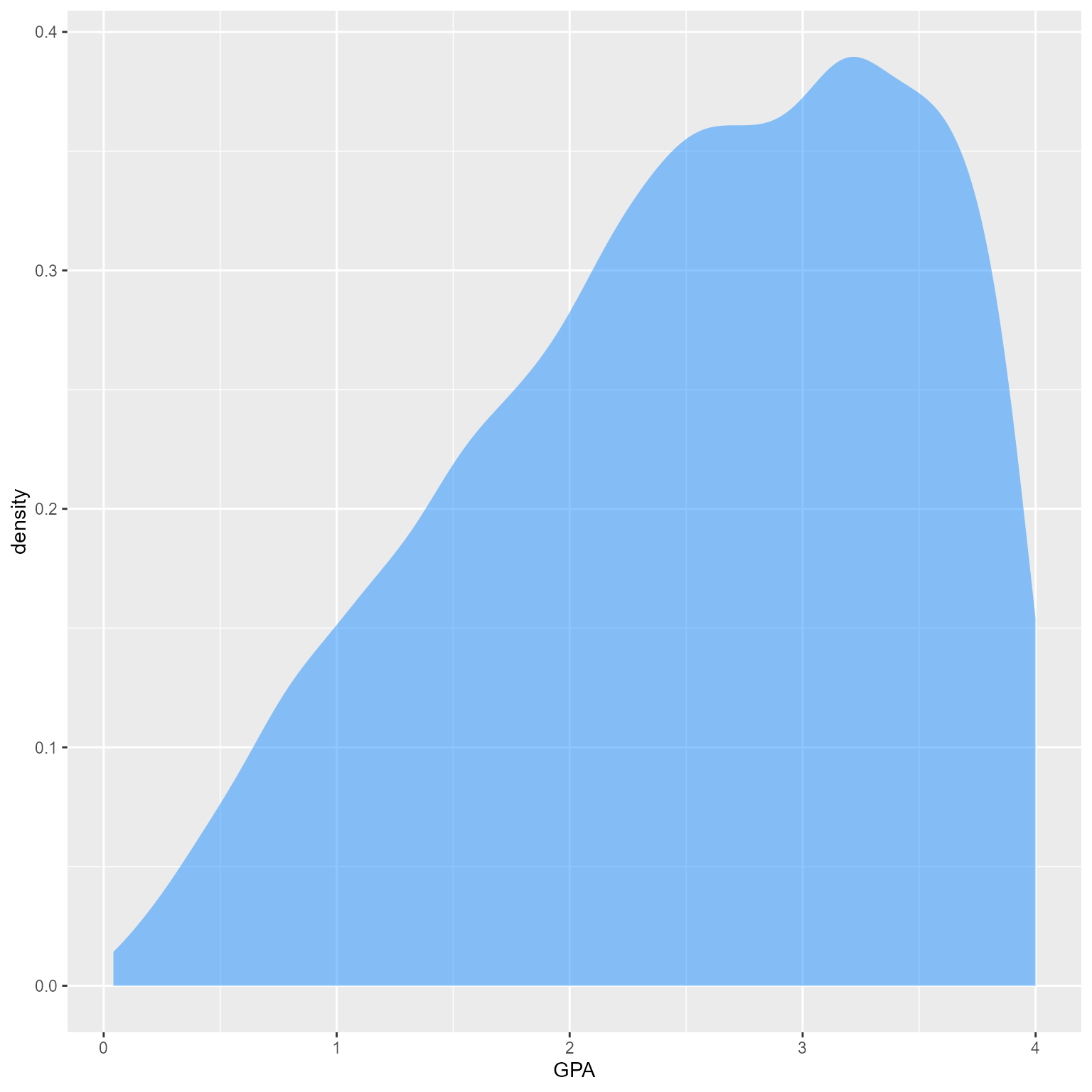

What is the distribution of Absences?

d %>% 
  count(Absences) %>% 
  ggplot(aes(Absences, n)) + 
  geom_col(fill = "dodgerblue", color = NA) +
  geom_text(aes(label = n), vjust = -.1)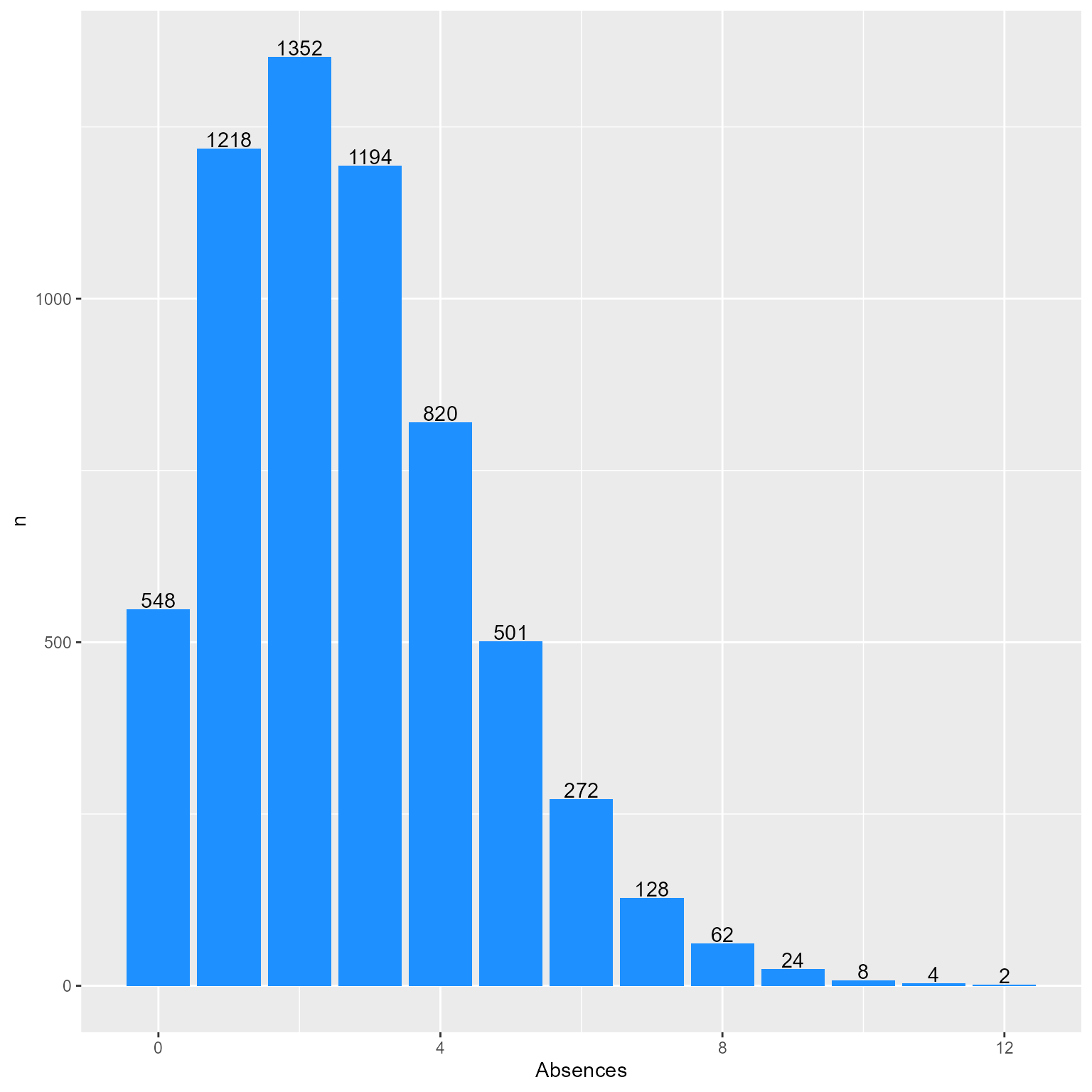

Dropout Rates Across Schools

d %>% 
  group_by(school_id, Intervention) %>% 
  summarise(Dropout = mean(Dropout)) %>% 
  ggplot(aes(Dropout)) +
  geom_density(aes(fill = Intervention), color = NA, alpha = 0.5) +
  labs(x = "School Dropout Rate")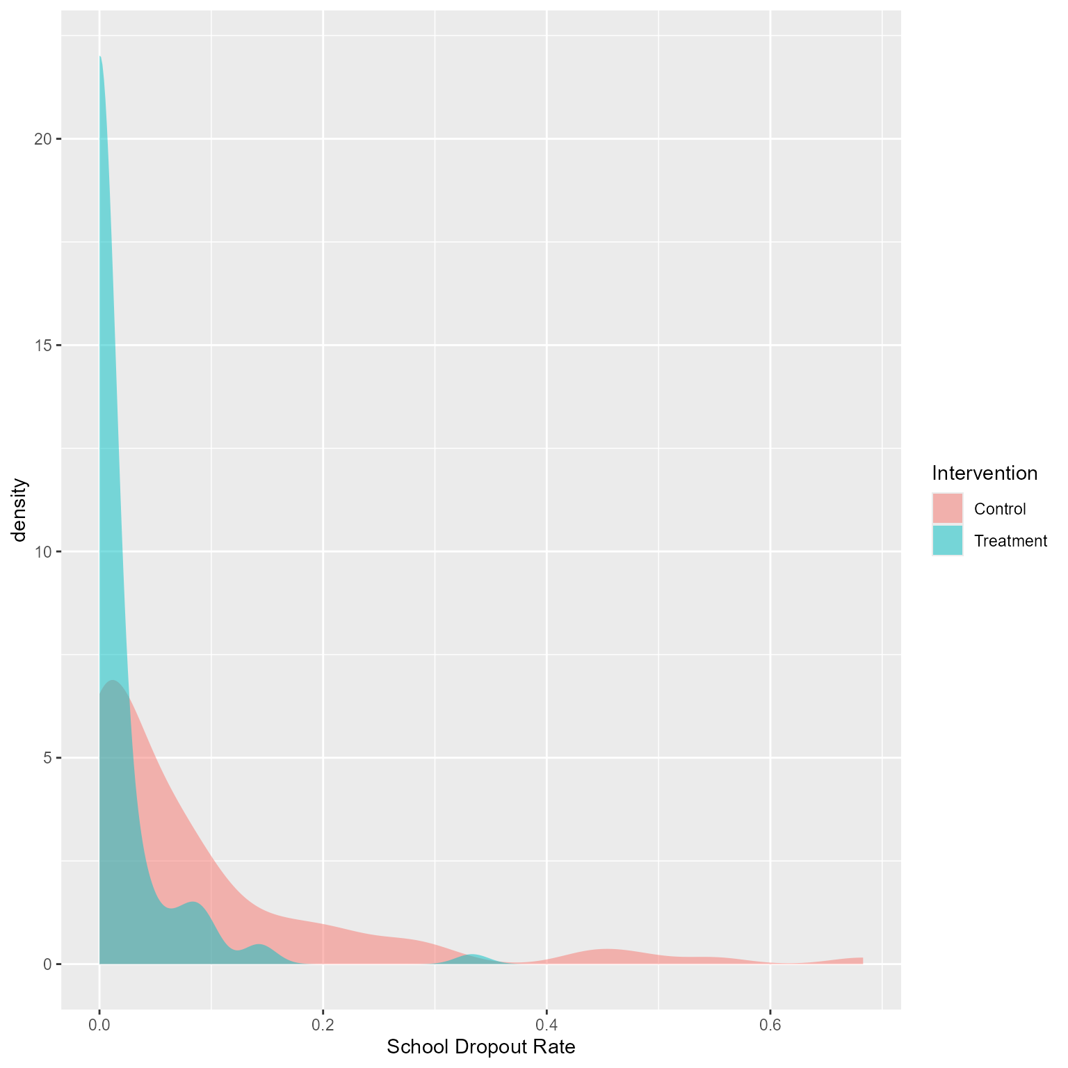

Let’s use the “glm” method in geom_smooth to get a rough sense of what a proper analysis is likely to show.

ggplot(d, aes(Absences, Dropout)) + 
  geom_jitter(aes(color = Intervention), 
              size = 0.3, 
              width = 0.2, 
              height = .015, 
              alpha = 0.5, 
              pch = 16) + 
  geom_smooth(aes(color = Intervention), 
              method = "glm", 
              method.args = list(family = "binomial"))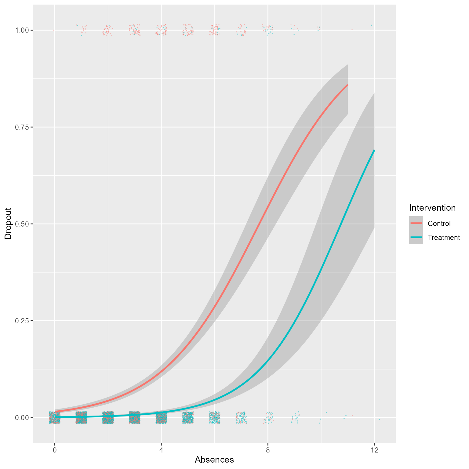

To me, that looks like a successful intervention! However, we did not do a proper analysis that accounted for the multilevel nature of the data.

Null model

The glmer function works exactly like lmer except that we must tell it which kind of generalized model we want. With binary outcomes, specify the binomial family. By default, it will do a logistic regression. You can specify probit regression with binomial(link = "probit"), if needed.

m0 <- glmer(Dropout ~ 1 + (1 | school_id), d, family = binomial())
summary(m0)

Generalized linear mixed model fit by maximum likelihood (Laplace
  Approximation) [glmerMod]
 Family: binomial  ( logit )
Formula: Dropout ~ 1 + (1 | school_id)
   Data: d

     AIC      BIC   logLik deviance df.resid 
    1827     1841     -912     1823     6131 

Scaled residuals: 
   Min     1Q Median     3Q    Max 
-1.375 -0.167 -0.070 -0.068  7.498 

Random effects:
 Groups    Name        Variance Std.Dev.
 school_id (Intercept) 4.46     2.11    
Number of obs: 6133, groups:  school_id, 200

Fixed effects:
            Estimate Std. Error z value Pr(>|z|)    
(Intercept)   -4.670      0.272   -17.2   <2e-16 ***
---
Signif. codes:  0 '***' 0.001 '**' 0.01 '*' 0.05 '.' 0.1 ' ' 1

performance(m0)

# Indices of model performance

AIC      |     AICc |      BIC | R2 (cond.) | R2 (marg.) |   ICC |  RMSE
------------------------------------------------------------------------
1827.186 | 1827.188 | 1840.629 |      0.576 |      0.000 | 0.576 | 0.185

AIC      | Sigma | Log_loss | Score_log | Score_spherical
---------------------------------------------------------
1827.186 | 1.000 |    0.121 |   -14.611 |           0.010

tab_model(m0)

	Dropout
Predictors	Odds Ratios	CI	p
(Intercept)	0.01	0.01 – 0.02	<0.001
Random Effects
σ²	3.29
τ₀₀ _{school_id}	4.46
ICC	0.58
N _{school_id}	200
Observations	6133
Marginal R² / Conditional R²	0.000 / 0.576

# If you want the raw coefficients (log-odds) instead of odds ratios
tab_model(m0, transform = NULL)

	Dropout
Predictors	Log-Odds	CI	p
(Intercept)	-4.67	-5.20 – -4.14	<0.001
Random Effects
σ²	3.29
τ₀₀ _{school_id}	4.46
ICC	0.58
N _{school_id}	200
Observations	6133
Marginal R² / Conditional R²	0.000 / 0.576

We can see from the ICC (or conditional R²) that 57.6% of the variance in dropout rate is explained by the grouping variable, school_id.

First L1 predictor: Absences

Let’s add to the null model using the update function.

m1 <- update(m0, . ~ . + Absences)
# Does this model fit better than the null model?
anova(m0,m1)

Data: d
Models:
m0: Dropout ~ 1 + (1 | school_id)
m1: Dropout ~ (1 | school_id) + Absences
   npar  AIC  BIC logLik deviance Chisq Df Pr(>Chisq)    
m0    2 1827 1841   -912     1823                        
m1    3 1371 1391   -682     1365   459  1     <2e-16 ***
---
Signif. codes:  0 '***' 0.001 '**' 0.01 '*' 0.05 '.' 0.1 ' ' 1

# Overall numbers
summary(m1)

Generalized linear mixed model fit by maximum likelihood (Laplace
  Approximation) [glmerMod]
 Family: binomial  ( logit )
Formula: Dropout ~ (1 | school_id) + Absences
   Data: d

     AIC      BIC   logLik deviance df.resid 
    1370     1391     -682     1364     6130 

Scaled residuals: 
   Min     1Q Median     3Q    Max 
-6.212 -0.097 -0.033 -0.015 17.443 

Random effects:
 Groups    Name        Variance Std.Dev.
 school_id (Intercept) 9.59     3.1     
Number of obs: 6133, groups:  school_id, 200

Fixed effects:
            Estimate Std. Error z value Pr(>|z|)    
(Intercept)  -9.0916     0.5889   -15.4   <2e-16 ***
Absences      0.8777     0.0537    16.4   <2e-16 ***
---
Signif. codes:  0 '***' 0.001 '**' 0.01 '*' 0.05 '.' 0.1 ' ' 1

Correlation of Fixed Effects:
         (Intr)
Absences -0.687

# Performance metrics
performance(m1)

# Indices of model performance

AIC      |     AICc |      BIC | R2 (cond.) | R2 (marg.) |   ICC |  RMSE
------------------------------------------------------------------------
1370.510 | 1370.514 | 1390.674 |      0.788 |      0.171 | 0.745 | 0.152

AIC      | Sigma | Log_loss | Score_log | Score_spherical
---------------------------------------------------------
1370.510 | 1.000 |    0.080 |      -Inf |           0.010

# Automated report
report(m1)

We fitted a logistic mixed model (estimated using ML and Nelder-Mead optimizer)
to predict Dropout with Absences (formula: Dropout ~ Absences). The model
included school_id as random effect (formula: ~1 | school_id). The model's
total explanatory power is substantial (conditional R2 = 0.79) and the part
related to the fixed effects alone (marginal R2) is of 0.17. The model's
intercept, corresponding to Absences = 0, is at -9.09 (95% CI [-10.25, -7.94],
p < .001). Within this model:

  - The effect of Absences is statistically significant and positive (beta =
0.88, 95% CI [0.77, 0.98], p < .001; Std. beta = 1.63, 95% CI [1.44, 1.83])

Standardized parameters were obtained by fitting the model on a standardized
version of the dataset. 95% Confidence Intervals (CIs) and p-values were
computed using a Wald z-distribution approximation.

# Nice table
tab_model(m1)

	Dropout
Predictors	Odds Ratios	CI	p
(Intercept)	0.00	0.00 – 0.00	<0.001
Absences	2.41	2.17 – 2.67	<0.001
Random Effects
σ²	3.29
τ₀₀ _{school_id}	9.59
ICC	0.74
N _{school_id}	200
Observations	6133
Marginal R² / Conditional R²	0.171 / 0.788

# Fixed effect plot
sjPlot::plot_model(m1, type = "pred", terms = "Absences")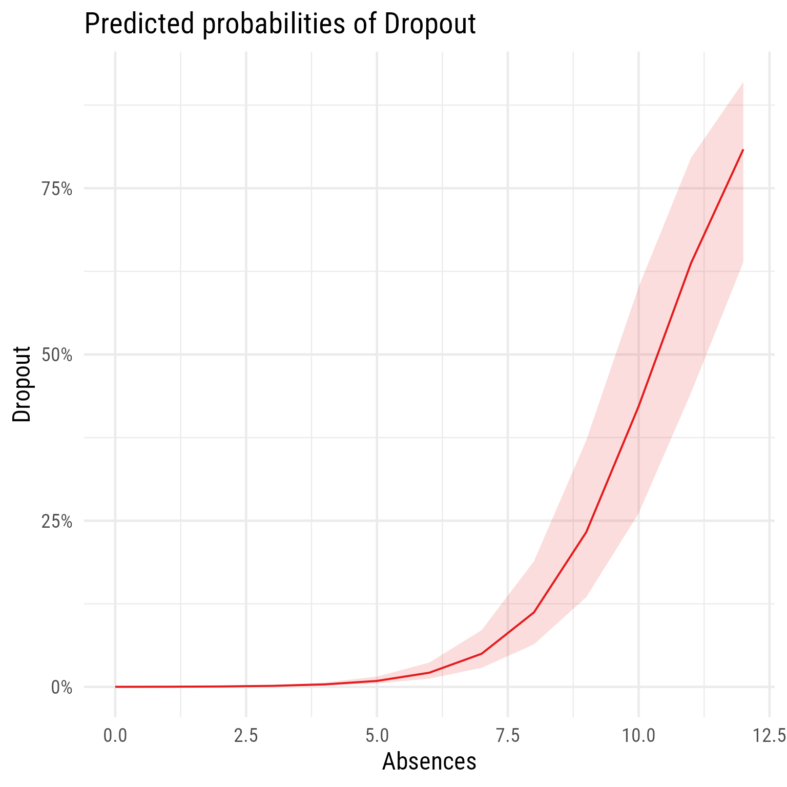

Second L1 predictor: GPA

Question 1

Add the GPA variable as a predictor to a model called m2. Conduct and interpret your analyses, documenting whether the GPA is a significant predictor of dropout rate.

This plot might aid interpretation.

sjPlot::plot_model(m2, 
                   type = "pred", 
                   terms = c("Absences", 
                             "GPA [0,2,4]"))

L2 predictor: Intervention

Question 2

Add the Intervention variable as a predictor to a model called m3. Conduct and interpret your analyses, documenting whether the intervention succeeded in reducing the dropout rate.

This plot might aid interpretation.

sjPlot::plot_model(m3, 
                   type = "pred", 
                   terms = c("Absences", 
                             "GPA [0,2,4]", 
                             "Intervention"))

Question 3

What additional analyses might you conduct with these data? Try testing at least one more model that makes sense to you and write your conclusions.