Multilevel Modeling of Longitudinal Data in R

Advanced Data Analysis (EDUC 8825)

Published

March 11, 2025

Longitudinal data analysis refers to the examination of how variables change over time, typically within individuals. Multilevel modeling allows us to study “unbalanced” longitudinal data in which not everyone has the same number of measurements.

In clustered data, the lowest level is typically a person, with higher levels referring to groups of people. With longitudinal data, the person is typically level 2, and level 1 is a measurement occasion associated with a specific instance in time.

With multilevel approaches to longitudinal data, data for each person fits on multiple rows with each measurement instance on its own row as seen in Table 1.

person_id time x y
1 0 6 5
1 1 7 6
1 2 10 7
2 0 14 2
2 1 18 3
2 2 20 5
Table 1: Longitudinal data with multiple rows per person

Specifying when the time variable equals 0 becomes increasingly important with complex longitudinal model because it influences the interpretation of other coefficients in the model. If there are interaction effects or polynomial effects, the lower-order effects refer to the effect of the variable when all other predictors are 0. Thus, we try to mark time such that T0 (when time = 0) is meaningful. For example, T0 is often simply the first measurement occasion. T0 could be the point at which an important event occurs, such as the onset of an intervention. In such cases, measurements before the intervention are marked as negative (Time = −3, −2, −1, 0, 1, 2, …).

Time does not have to be marked as integers, not everyone needs to be measured at the same times, and measurements do not necessarily need to occur at exactly T0. For person 1, the measurements could be at Time = −2.1 minutes, +5.3 minutes, and +44.2 minutes. For person 2, the measurements could be at Time = −8.8 minutes, −6.0 minutes, +10.1 minutes, and +10.5 minutes.

Hypothetical Longitudinal Study of Reading Comprehension

Suppose we are measuring how schoolchildren’s reading comprehension changes over time. We believe that reading comprehension (understanding of the text’s meaning) is influenced by Reading Decoding skills (correct identification of words). If we measure Reading Decoding skill at each occasion, it is a time-varying covariate at level 1.

Suppose we believe that children’s working memory capacity also is an important influence on reading comprehension. If we only measure working memory capacity once (typically at the beginning of the study), working memory capacity is a person-level covariate at level 2. Of course, if we had measured working memory capacity at each measurement occasion, it would be an additional time-varying covariate at level 1.

For the sake of demonstration, I am going to present a model in which Working Memory Capacity not only influences the initial level of Reading Comprehension, but it also has every possible cross-level interaction effect. In a real analysis, we would only investigate such effects if we had good theoretical reasons for doing so. Testing for every possible effect just because we can will dramatically increase our risk of “finding” spurious effects.

Level 1: Measurement Occasion

Every time a person is measured, we will call this a measurement occasion. In longitudinal studies, each measurement occasion is placed in its own data row.

\begin{align*} Y_{ti}&=b_{0i}+b_{1i}T_{ti}+b_{2i}RD_{ti}+e_{ti}\\ e_{ti}&\sim\mathcal{N}(0, \tau_1^2) \end{align*}

Variable Interpretation
Y_{ti} The measure of Reading Comprehension for person i at occasion (time) t.
RD_{ti} The measure of Reading Decoding at occasion t for person i.
T_{ti} How much time has elapsed at occasion t for person i.
b_{0i} The random intercept: The predicted Reading Comprehension for person i at time 0 (T0) if Reading Decoding = 0.
b_{1i} The random slope of Time: The rate of increase in Reading Comprehension for person i if Reading Decoding is held constant at 0.
b_{2i} The size of Reading Decoding’s association with Reading Comprehension for person i.
e_{ti} The deviation from expectations for Reading Comprehension at occasion t for person i. It represents the model’s failure to accurately predict Reading Comprehension at each measurement occasion.
\tau_1 The variance of e_{ti}

Level 2: Person

Predicting the Random Intercept (b_{0i}):
What Determines the Conditions at T0?

If Time and Reading Decoding = 0, what determines our prediction of Reading Comprehension?

b_{0i}=b_{00}+b_{01}WM_i+e_{0i}

Variable Interpretation
b_{0i} The random intercept: The predicted Reading Comprehension for person i at time 0 (T0) if Reading Decoding = 0.
WM_i The measurement of Working Memory Capacity for person i.
b_{00} The predicted value of Reading Comprehension when Time, Reading Decoding, and Working Memory = 0.
b_{01} Working Memory’s association with Reading Comprehension at T0 when Reading Decoding is 0.
e_{0i} Person i’s deviation from expectations for the random intercept. It represents the model’s failure to predict each person’s random intercept.

Predicting Time’s Random Slope:
What determines the effect of time (Grade)?

Suppose we believe that Reading Comprehension will, on average, increase over time for everyone, but the rate of increase will be faster for children with greater working memory capacity.

b_{1i}=b_{10}+b_{11}WM_i+e_{1i}

Variable Interpretation
b_{1i} The random slope of Time: The rate of increase in Reading Comprehension for person i if Reading Decoding is held constant at 0.
b_{10} The rate at which Reading Comprehension increases for each unit of time if both Reading Decoding and Working Memory are held constant at 0.
b_{11} Working Memory’s effect on the rate of Reading Comprehension’s change over time, after controlling for Reading Decoding (i.e., if Reading Decoding were held constant at 0). If positive, students with higher working memory should improve their Reading Comprehension ability faster than students with lower working memory.
e_{1i} Person i’s the deviation from expectations for the random slope for time. It represents the model’s failure to predict each person’s rate of increase in Reading Comprehension over time (after controlling for Reading Decoding).

Predicting Reading Decoding’s Random Slope:
What determines the effect of Reading Decoding?

Suppose that the effect of Reading Decoding on Reading Comprehension differs from person to person. Obviously, to comprehend text a person needs at least some ability to decode words. However, there is evidence that working memory helps a person make inferences in reading comprehension such that one can work around unfamiliar words and still derive meaning from the text. Thus, we might predict that higher Working Memory Capacity makes Reading Decoding a less important predictor of Reading Comprehension.

b_{2i}=b_{20}+b_{21}WM_i+e_{2i}

Variable Interpretation
b_{2i} The size of Reading Decoding’s association with Reading Comprehension for person i.
b_{20} The size of the association of Reading Decoding and Reading Comprehension when Working Memory is 0.
b_{21} The interaction effect of Working Memory and Reading Decoding. It represents how much the effect of Reading Decoding on Reading Comprehension changes for each unit of increase in Working Memory.
e_{2i} Person i’s the deviation from expectations for the random slope for Reading Decoding. It represents the model’s failure to predict the person-specific relationship between Reading Decoding and Reading Comprehension.

Level-2 Random Effects

The error terms at level 2 (e_{0i}, e_{1i}, \&~e_{2i}) have variances, and possibly covariances.

\begin{align*} \boldsymbol{e}_2&= \begin{bmatrix} e_{0i}\\ e_{1i}\\ e_{2i} \end{bmatrix}\\ \boldsymbol{e}_2&\sim\mathcal{N}\left(\boldsymbol{0},\boldsymbol{\tau}_2\right)\\ \boldsymbol{\tau}_2&= \begin{bmatrix} \tau_{2.00}\\ \tau_{2.10} & \tau_{2.11}\\ \tau_{2.20} & \tau_{2.21} & \tau_{2.22} \end{bmatrix} \end{align*}

Combined Equations

\begin{align} Y_{ti}&= \underbrace{b_{00}+b_{01}WM_i+u_{0i}}_{b_{0i}~\text{(Random Intercept)}}\\ &+(\underbrace{b_{10}+b_{11}WM_i+u_{1i}}_{b_{1i}~\text{(Random Slope for Time)}})T_{ti}\\ &+(\underbrace{b_{20}+b_{21}WM_i+u_{2i}}_{b_{2i}~\text{(Random Slope for RD)}})RD_{ti}\\ &+e_{ti} \end{align}

An equation aligned to the lmer formula:

\begin{align} Y_{ti}&=b_{00}\\ &+\underbrace{b_{01}WM_i+b_{10}T_{ti}+b_{20}RD_{ti}}_{\text{Simple Slopes (when other predictors = 0)}}\\ &+\underbrace{b_{11}T_{ti}WM_i+b_{21}RD_{ti}WM_i}_{\text{Interactions}}\\ &+\underbrace{e_{0i}+e_{1i}T_{ti}+e_{2i}RD_{ti}}_{\text{L2 Random Effects}}\\ &+e_{ti} \end{align}

Here is the model as a lmer formula:

reading_comprehension~1+
working_memory+time+reading_decoding+
time:working_memory+reading_decoding:working_memory+
(1+time+reading_decoding | person_id)

A simplified version would look like this:

reading_comprehension~
working_memory * time + 
working_memory * reading_decoding +
(time+reading_decoding | person_id)

Simulate longitudinal data

I am going to simulate a longitudinal observational study of these three variables.

To make things simple, suppose that Reading Decoding also grows over time like so:

RD_{ti}=6+2T_{ti}+.5WM_{ti}+e_{ti}\\ e\sim\mathcal{N}(0, 1^2)

Simulate Level-2 Data (Person Level)

We begin at level 2 by setting the sample size, the fixed effects, the level-2 random effect covariance matrix (\boldsymbol{\tau}), and

We can simulate Working Memory Capacity as a standard normal variable.

library(tidyverse)
library(lme4)
library(sjPlot)
set.seed(123456)
# Sample size
n_person <- 2000

# Number of occasions
n_occasions <- 6

# Fixed effects
b_00 <- 60 # Fixed intercept
b_01 <- 10 # simple main effect of working memory
b_10 <- 50 # simple main effect of time (Grade)
b_11 <- 5 # time * working memory interaction
b_20 <- 8 # simple main effect of reading decoding
b_21 <- -0.9 # reading decoding * working memory interaction

# Standard deviations of level-2 random effects
e_sd <- c(e0i = 50, # sd of random intercept
          e1i = 1.7, # sd of random slope for time
          e2i = 1.8) # sd of random slope for reading decoding

# Correlations among level-2 random effects
e_cor <- c(1,
           0, 1,
           0, 0, 1) %>% 
  lavaan::lav_matrix_lower2full(.)

# level-2 random effects covariance matrix
tau_2 <- lavaan::cor2cov(R = e_cor, 
                       sds = e_sd, 
                       names = names(e_sd))

# simulate level-2 random effects
e_2 <- mvtnorm::rmvnorm(n_person, 
                      mean = c(e0i = 0, e1i = 0, e2i = 0), 
                      sigma = tau_2) %>% 
  as_tibble()

# Simulate level-2 data and coefficients
d_level2 <- tibble(person_id = factor(1:n_person),
                   n_occasions = n_occasions,
               working_memory = rnorm(n_person)) %>% 
  bind_cols(e_2) %>% 
  mutate(b_0i = b_00 + b_01 * working_memory + e0i,
         b_1i = b_10 + b_11 * working_memory + e1i,
         b_2i = b_20 + b_21 * working_memory + e2i)

d_level2
# A tibble: 2,000 × 9
   person_id n_occasions working_memory    e0i     e1i     e2i  b_0i  b_1i  b_2i
   <fct>           <dbl>          <dbl>  <dbl>   <dbl>   <dbl> <dbl> <dbl> <dbl>
 1 1                   6        -1.22    41.7  -0.469  -0.639   89.5  43.4  8.46
 2 2                   6         1.20     4.37  3.83    1.50    76.3  59.8  8.43
 3 3                   6        -0.956   65.6   4.25    2.10   116.   49.5 11.0 
 4 4                   6        -0.746  -21.3  -1.69   -2.01    31.2  44.6  6.67
 5 5                   6        -1.64    -2.79  2.00    1.90    40.9  43.8 11.4 
 6 6                   6        -0.0452   2.88 -1.25    1.67    62.4  48.5  9.72
 7 7                   6        -0.933   83.4   0.951  -1.36   134.   46.3  7.48
 8 8                   6        -0.291   62.8   0.0654  0.341  120.   48.6  8.60
 9 9                   6         1.36    23.1  -0.727   0.0299  96.7  56.1  6.81
10 10                  6         0.311   35.2   1.65   -1.12    98.4  53.2  6.60
# ℹ 1,990 more rows

Simulate Level-1 Data (Occasion Level)

Let’s say that our measurement of our level-1 variables occurs at the beginning of each Grade starting in Kindergarten (i.e., Grade 0) and continues every year until fifth grade. Our measurement of working memory capacity occurs once—at the beginning of Kindergarten.

# level-1 sd
tau_1 <- 15 ^ 2

d_level1 <- d_level2 %>% 
  uncount(n_occasions) %>% 
  group_by(person_id) %>% 
  mutate(Grade = row_number() - 1) %>% 
  ungroup() %>% 
  mutate(reading_decoding = 6 + 2 * Grade + .5 * working_memory + rnorm(nrow(.)),
         e_ti = rnorm(nrow(.), 0, sd = sqrt(tau_1)), 
         reading_comprehension = b_0i + b_1i * Grade + b_2i * reading_decoding + e_ti) %>% 
  arrange(Grade, reading_comprehension) %>% 
  mutate(person_id = fct_inorder(person_id)) %>% 
  arrange(person_id, Grade)

d_level1
# A tibble: 12,000 × 12
   person_id working_memory   e0i   e1i    e2i   b_0i  b_1i  b_2i Grade
   <fct>              <dbl> <dbl> <dbl>  <dbl>  <dbl> <dbl> <dbl> <dbl>
 1 12                 0.557 -137. -1.92 -1.55   -71.9  50.9  5.95     0
 2 12                 0.557 -137. -1.92 -1.55   -71.9  50.9  5.95     1
 3 12                 0.557 -137. -1.92 -1.55   -71.9  50.9  5.95     2
 4 12                 0.557 -137. -1.92 -1.55   -71.9  50.9  5.95     3
 5 12                 0.557 -137. -1.92 -1.55   -71.9  50.9  5.95     4
 6 12                 0.557 -137. -1.92 -1.55   -71.9  50.9  5.95     5
 7 918               -1.87  -151.  2.37 -0.284 -109.   43.0  9.40     0
 8 918               -1.87  -151.  2.37 -0.284 -109.   43.0  9.40     1
 9 918               -1.87  -151.  2.37 -0.284 -109.   43.0  9.40     2
10 918               -1.87  -151.  2.37 -0.284 -109.   43.0  9.40     3
# ℹ 11,990 more rows
# ℹ 3 more variables: reading_decoding <dbl>, e_ti <dbl>,
#   reading_comprehension <dbl>

Notes on the code from above:

Code Interpretation
uncount(n_occasions) Make copies of each row in d_level2 according to what value is in n_occasions, which in this case is 6 in every row. Thus, the 6 copies of each row d_level2 are made.
group_by(person_id) “I’m about to do something to groups of rows defined by person_id.”
mutate(Grade = row_number() - 1) Create a variable called Grade by taking the row number of each group defined by person_id and subtract 1. Because there are 6 rows per person, the values within each person will be 0, 1, 2, 3, 4, 5
ungroup() Stop computing things by group and compute variables the same way for the whole tibble.

If the data were real, and I wanted to test the hypothesized model, I would run this code:

library(lme4)
fit <- lmer(reading_comprehension ~ 1 + Grade * working_memory  + reading_decoding*working_memory + (1 + Grade + reading_decoding || person_id), data = d_level1 ) 
summary(fit)
Linear mixed model fit by REML ['lmerMod']
Formula: 
reading_comprehension ~ 1 + Grade * working_memory + reading_decoding *  
    working_memory + ((1 | person_id) + (0 + Grade | person_id) +  
    (0 + reading_decoding | person_id))
   Data: d_level1

REML criterion at convergence: 109220.4

Scaled residuals: 
    Min      1Q  Median      3Q     Max 
-3.3829 -0.5871 -0.0044  0.5850  3.0921 

Random effects:
 Groups      Name             Variance Std.Dev.
 person_id   (Intercept)      2460.172 49.600  
 person_id.1 Grade               2.241  1.497  
 person_id.2 reading_decoding    3.517  1.875  
 Residual                      222.953 14.932  
Number of obs: 12000, groups:  person_id, 2000

Fixed effects:
                                Estimate Std. Error t value
(Intercept)                      60.7239     1.4854  40.880
Grade                            50.1376     0.3272 153.240
working_memory                   10.7375     1.4716   7.296
reading_decoding                  7.9683     0.1640  48.599
Grade:working_memory              5.5824     0.3233  17.265
working_memory:reading_decoding  -1.0912     0.1620  -6.734

Correlation of Fixed Effects:
            (Intr) Grade  wrkng_ rdng_d Grd:w_
Grade        0.587                            
workng_mmry  0.045  0.043                     
redng_dcdng -0.621 -0.932 -0.039              
Grd:wrkng_m  0.042 -0.010  0.584  0.012       
wrkng_mmr:_ -0.039  0.012 -0.619 -0.018 -0.931

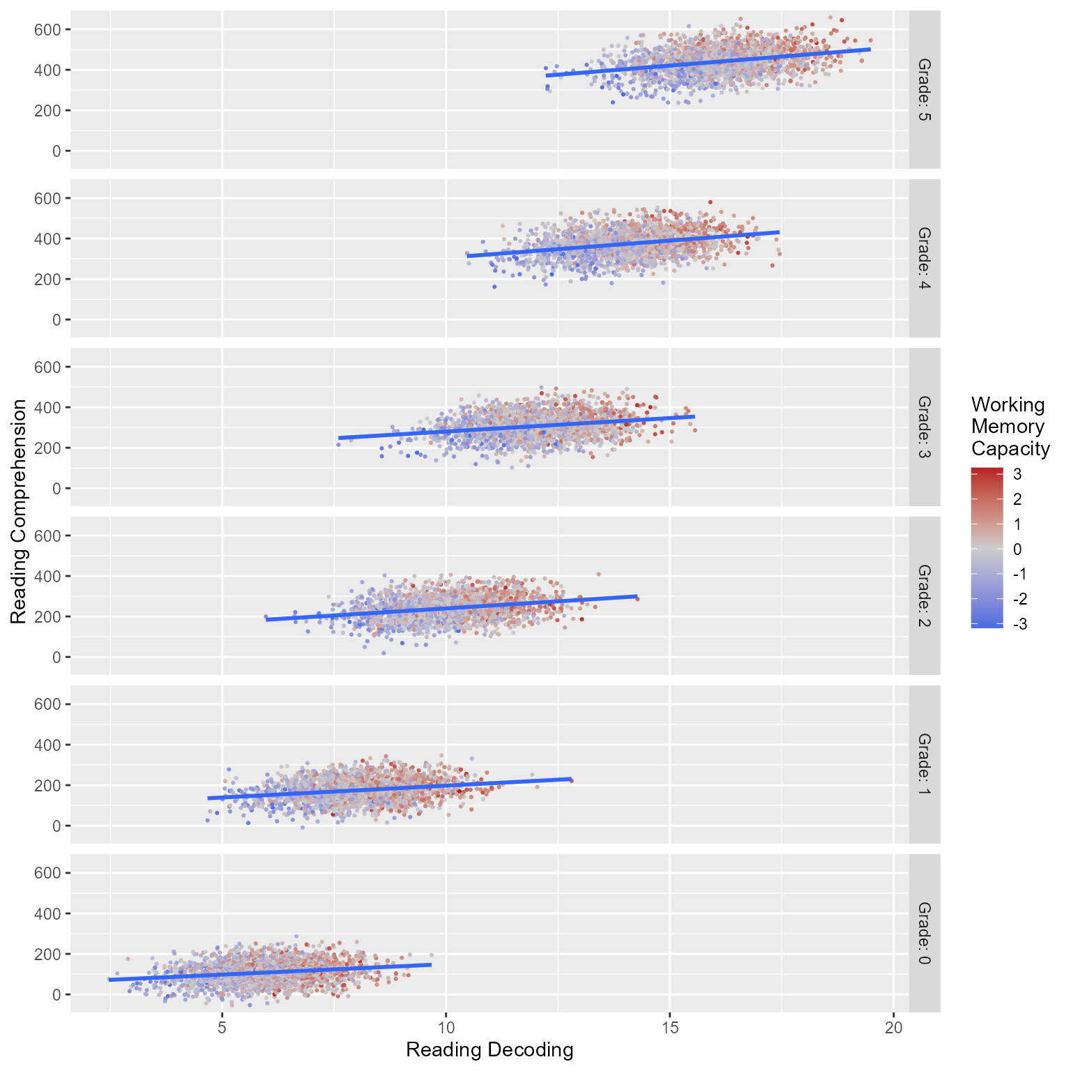
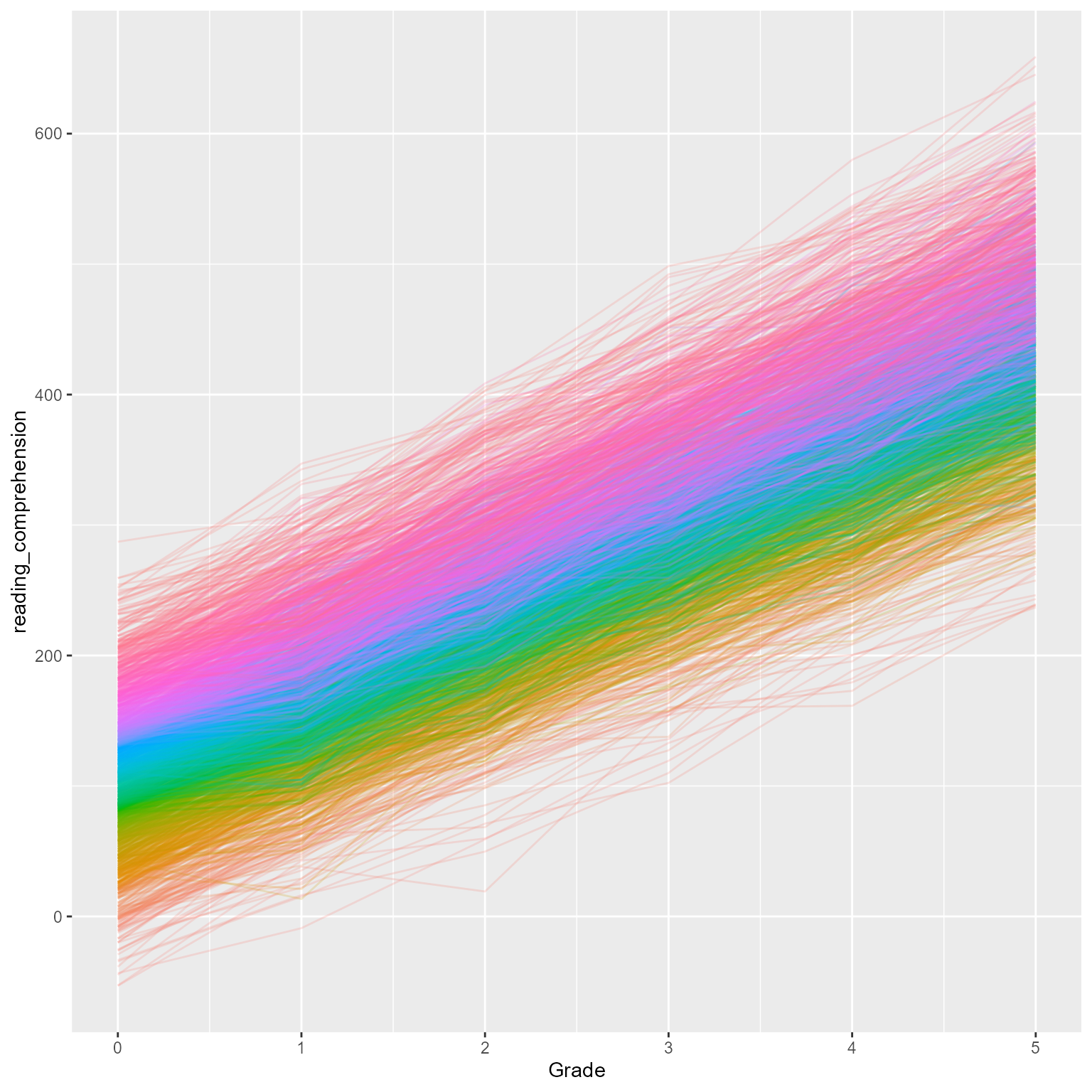
Figure 1 plots the observed data, in which we can see that both reading decoding and reading comprehension increase across grade and that high working memory is associated with higher levels of the reading variables.

ggplot(d_level1, aes(reading_decoding, reading_comprehension, color = working_memory)) + 
  geom_point(pch = 16, size = .75) + 
  geom_smooth(method = "lm", formula = y ~ x) +
  facet_grid(rows = vars(Grade), as.table = F, labeller = label_both) +
  scale_color_gradient2("Working\nMemory\nCapacity", mid = "gray80", low = "royalblue", high = "firebrick") + 
  labs(x = "Reading Decoding", y = "Reading Comprehension")
Figure 1: Reading Decoding Predicting

These effects might be easier to see in an animated plot like Figure 2.

library(gganimate)
ggplot(d_level1 %>% mutate(Grade = factor(Grade)), aes(reading_decoding, reading_comprehension, color = working_memory)) + 
  geom_point(pch = 16, size = .75) + 
  geom_smooth(method = "lm", formula = y ~ x) +
  # facet_grid(rows = vars(Grade), as.table = F, labeller = label_both) +
  scale_color_gradient2("Working\nMemory\nCapacity", mid = "gray80", low = "royalblue", high = "firebrick") + 
  scale_x_continuous("Reading Decoding", limits = c(0,20)) +
  scale_y_continuous("Reading Comprehension") + 
  transition_states(Grade) + 
  labs(title = 'Grade: {closest_state}') +
  coord_fixed(1 / 40)
Figure 2: Reading Decoding Predicting

If you need to plot interaction effects, and you want to make your life much, much easier, use the plot_model function from the sjPlot package.

In the terms parameter of the plot_model function, the first term is what goes on the x-axis. The second term is the moderator variable that shows up as lines with different colors. By default, it plots values at plus or minus 1 standard deviation, but you can specify any values you wish.

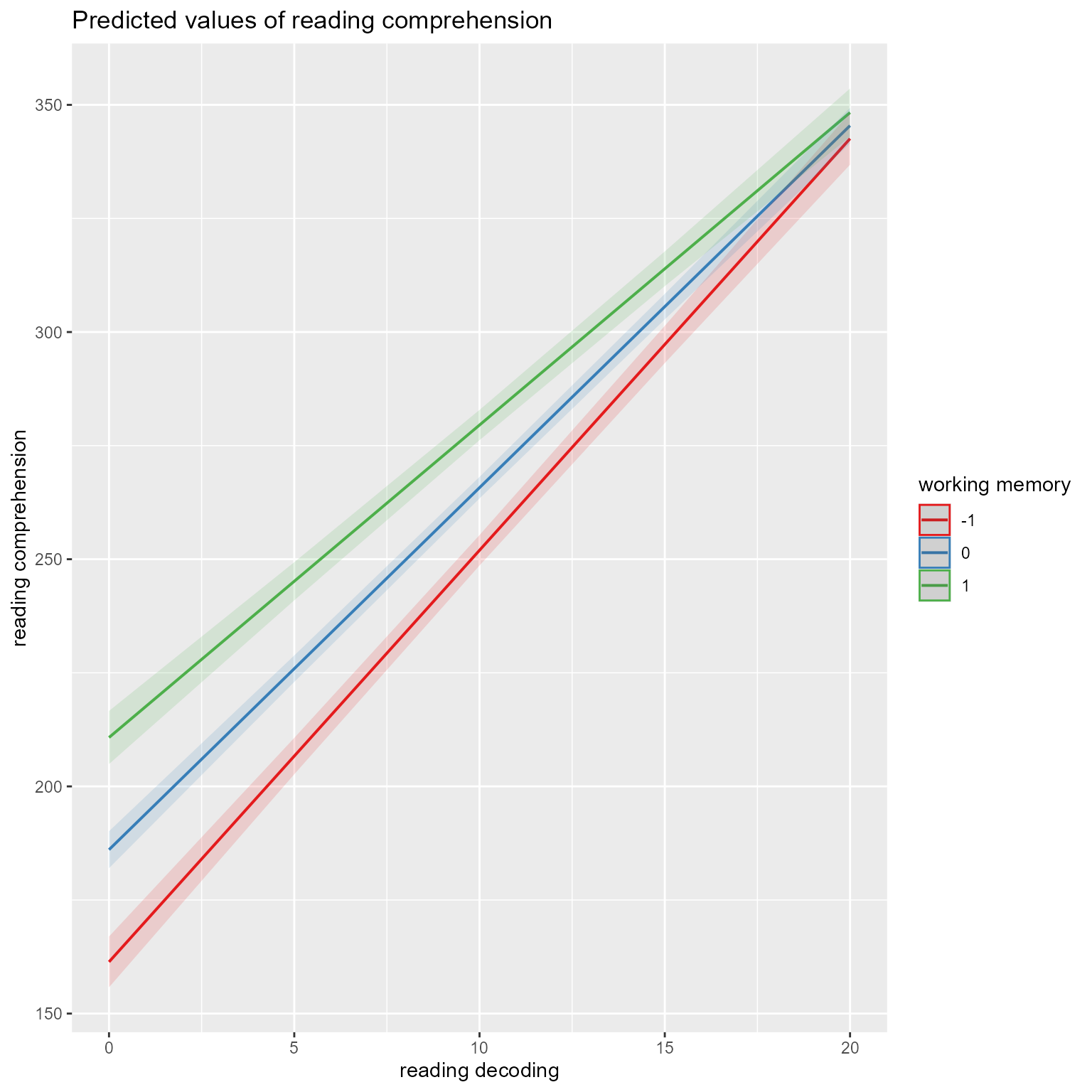
In Figure 3, it can be seen that reading decoding is related to reading comprehension but the strength of that relation depends on working memory. The effects of reading decoding are increasingly strong as working memory decreases.

library(sjPlot)
# Simple slopes of reading decoding at different levels of working memory (collapsing across grade)
plot_model(fit, 
           type = "pred", 
           terms = c("reading_decoding", "working_memory [-1, 0, 1]")) 
Figure 3: The Effects of Reading Decoding Are Moderated by Working Memory

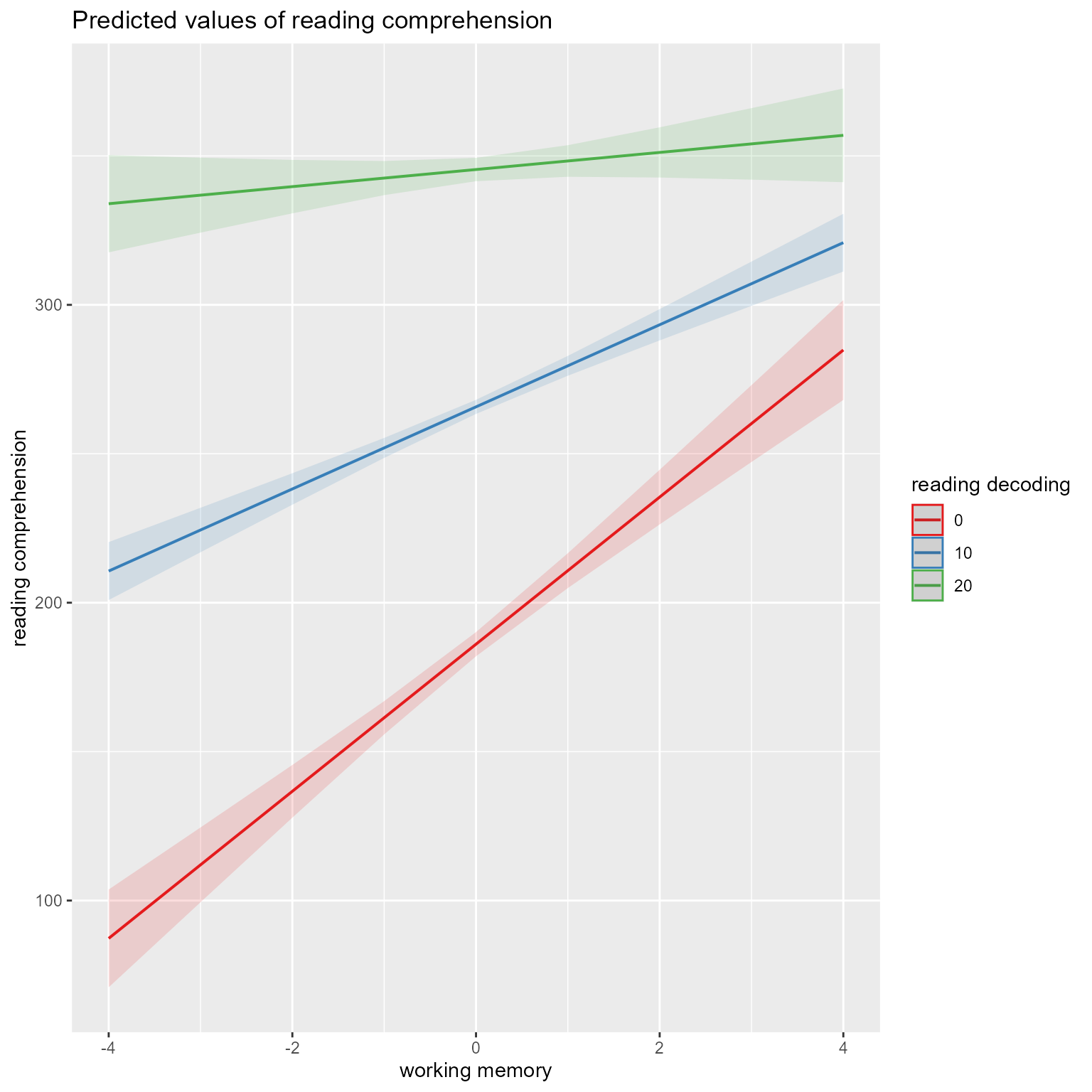
Another way to think about the interaction is to say that for poor decoders working memory strongly predicts reading comprehension. By contrast, for strong decoders, working memory is a weak predictor. In Figure 4, we are viewing the same interaction seen Figure 3 but we have flipped the x-axis and the color-facet. There is no new information here, but it helps to see the finding from different vantage points.

library(sjPlot)
# Simple slopes of working memory at different levels of reading decoding (collapsing across grade)
plot_model(fit, 
           type = "pred", 
           terms = c("working_memory", "reading_decoding [0, 10, 20]")) 
Figure 4: The Effects of Working Memory Depend on Reading Decoding

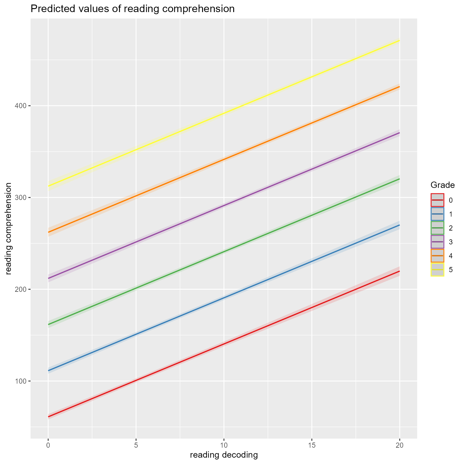
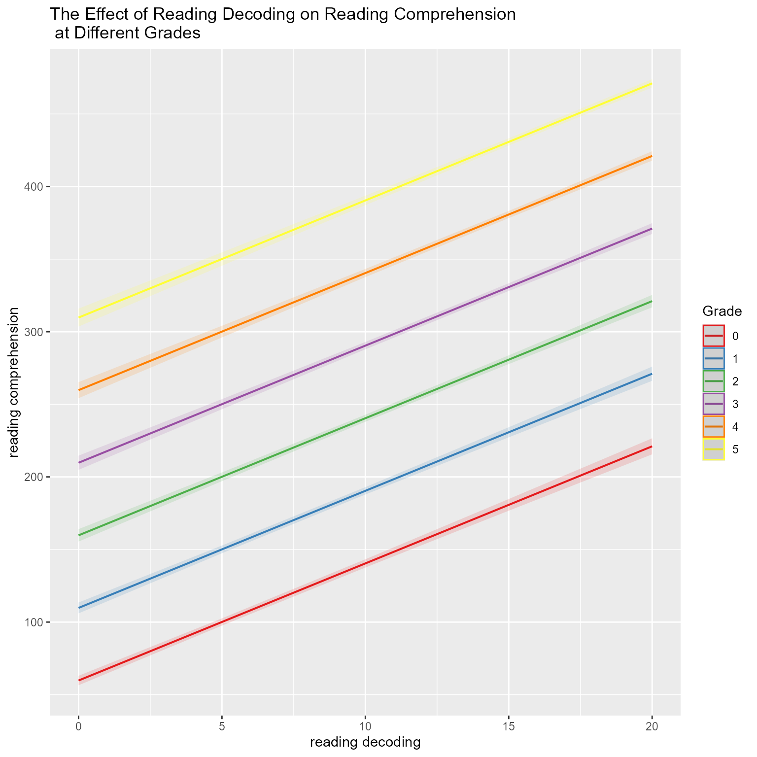
In Figure 5, we can view the simple slopes of reading decoding at different levels of grade (collapsing across working memory). Because the simple slopes are parallel, it appears that the effect of reading decoding is constant across grades.

plot_model(fit, 
           type = "pred", 
           terms = c("reading_decoding", "Grade"))
Figure 5: The Effects of Reading Decoding at Different Grades

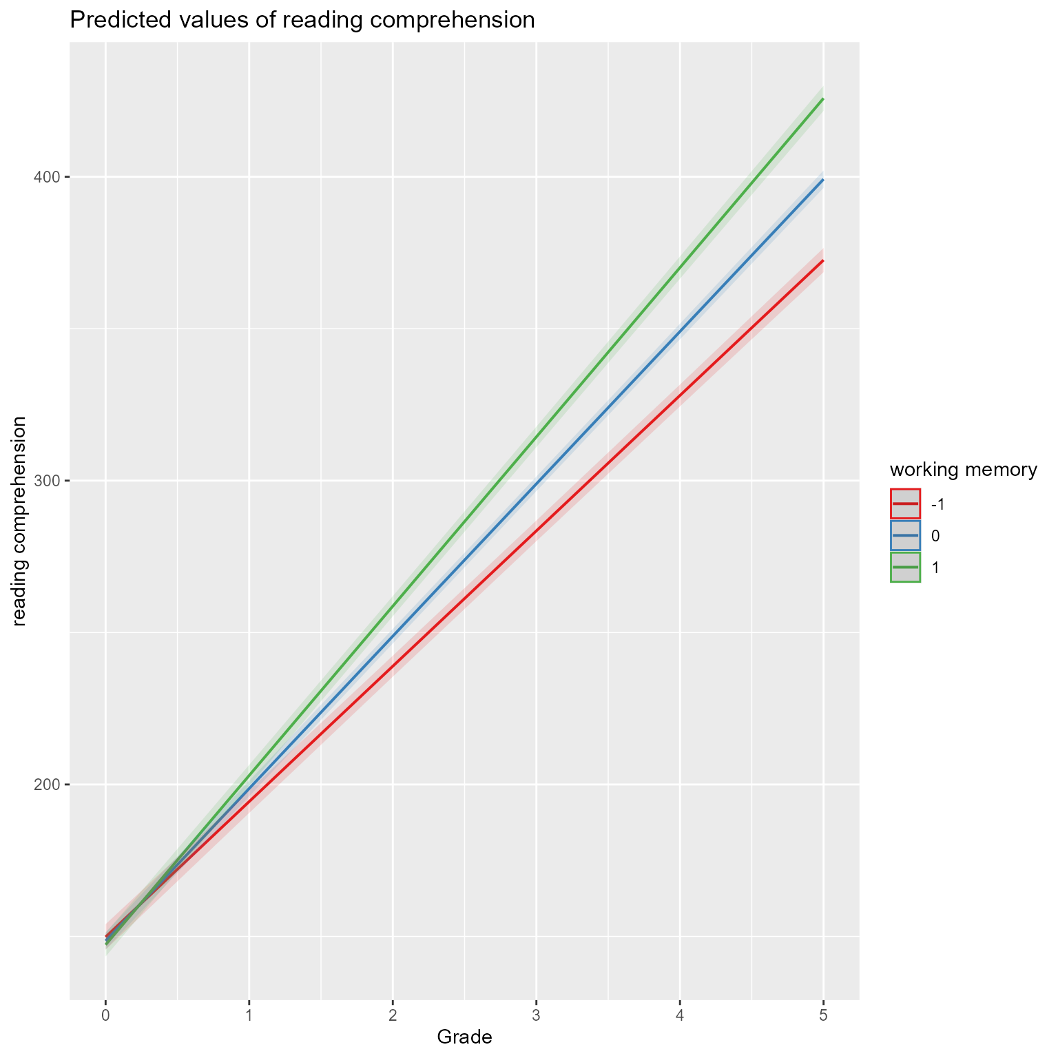
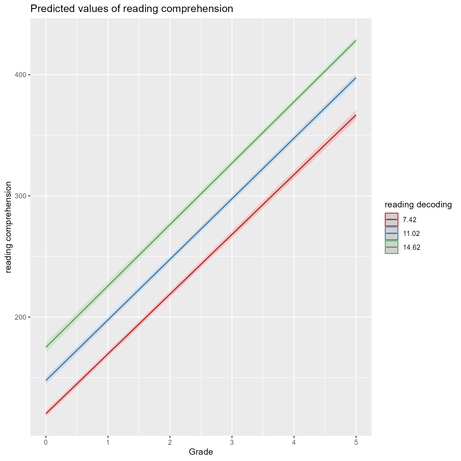
In Figure 6, we see that reading comprehension grows faster for students with higher working memory than for students with lower working memory.

plot_model(fit, 
           type = "pred", 
           terms = c("Grade", "working_memory [-1, 0, 1]"))
Figure 6: The Growth of Reading Comprehension Across Grade at Different Levels of Working Memory

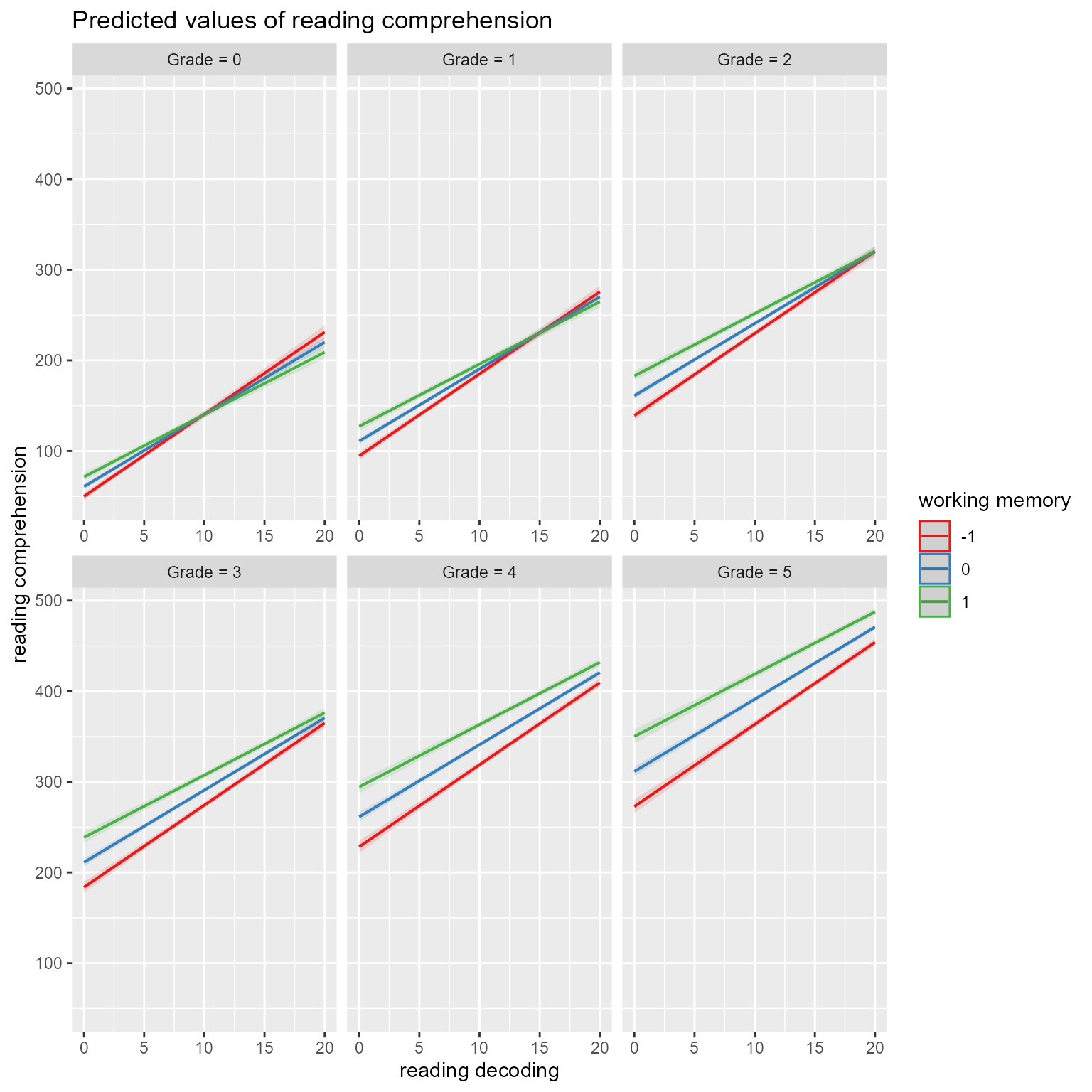
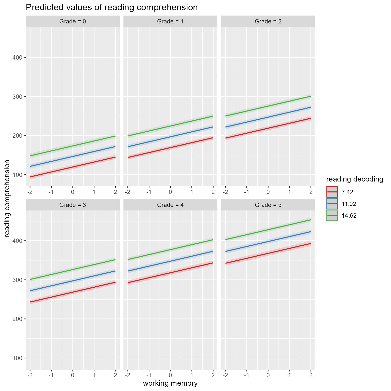
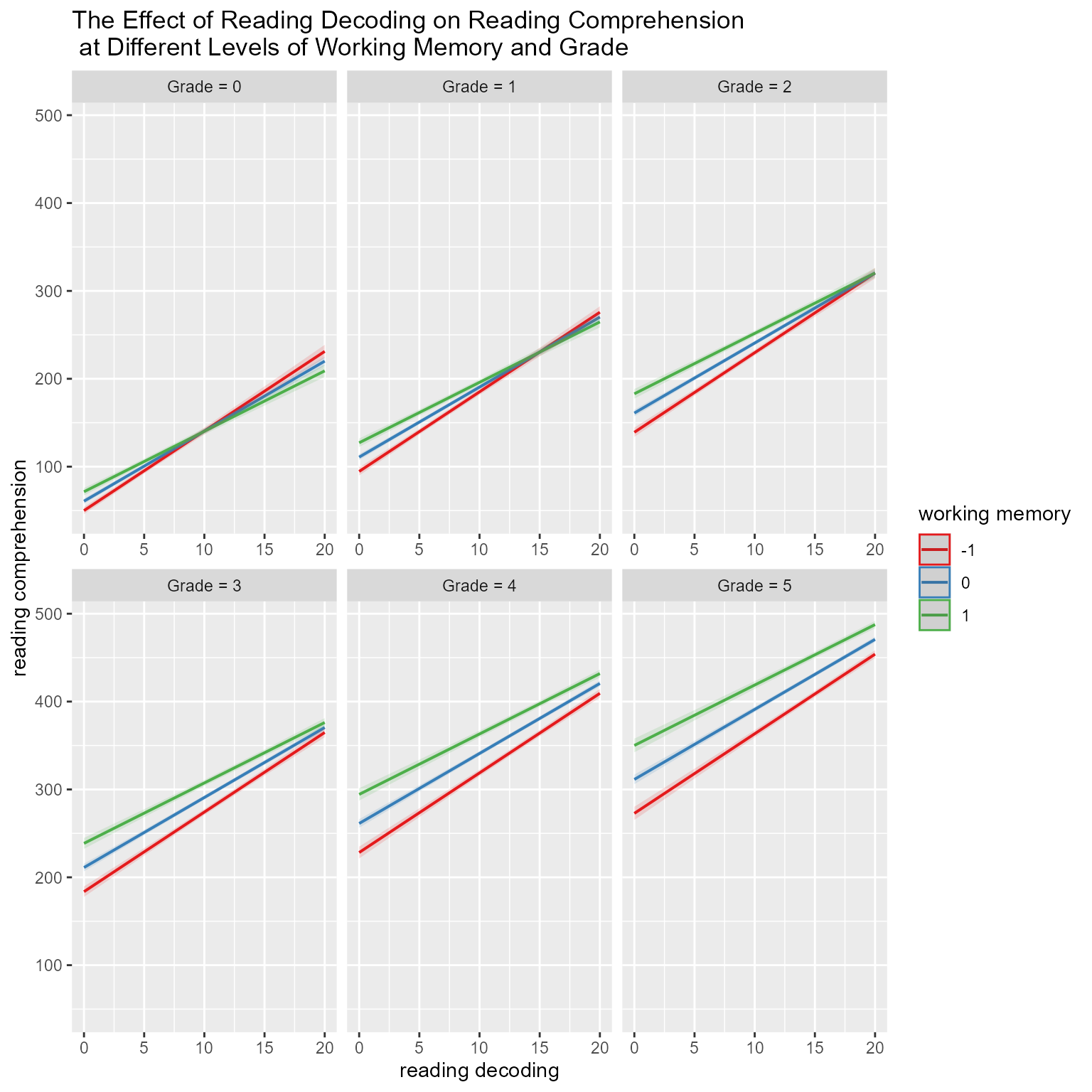
In Figure 7, we see the effects of reading decoding, working memory, and grade simultaneously. It appears that reading decoding’s effect is stronger for students with lower working memory but that the effect of working memory becomes increasingly strong across grades.

# Show simple slopes of reading decoding at different levels of grade and working memory
plot_model(fit, 
           type = "pred", 
           terms = c("reading_decoding", "working_memory [-1, 0, 1]", "Grade [0:5]"))
Figure 7: The Effect of Reading Decoding on Reading Comprehensionat Different Levels of Working Memory and Grade

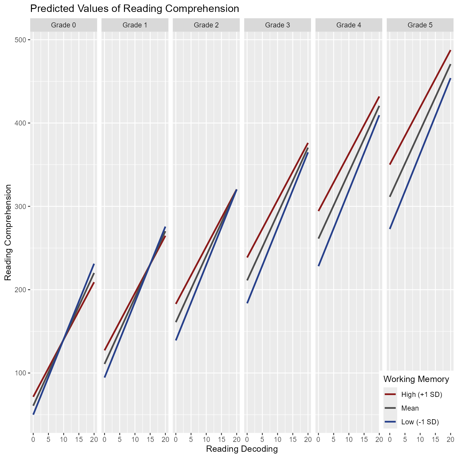
I can’t tell you how much trouble functions like plot_model will save you. I don’t care to admit how many hours of my life have been spent making interaction plots. Of course, ggplot2 made my coding experience much simpler than it used to to be. I mainly use sjPlot to make quick plots. If I needed to make a publication-ready plot, I would probably use code like Figure 8.

# Make predicted values at each unique combination of predictor variables
d_predicted <- crossing(Grade = 0:5,
                        working_memory = c(-1, 0, 1),
                        reading_decoding = c(0, 20)) %>%
  mutate(reading_comprehension = predict(fit, newdata = ., re.form = NA),
         working_memory = factor(working_memory,
                                 levels = c(1, 0,-1),
                                 labels = c("High (+1 SD)",
                                            "Mean",
                                            "Low (-1 SD)")))

ggplot(d_predicted,
       aes(x = reading_decoding, 
           y = reading_comprehension, 
           color = working_memory)) +
  geom_line(aes(group = working_memory), size = 1) +
  facet_grid(cols = vars(Grade), 
             labeller = label_bquote(cols = Grade ~ .(Grade))) +
  scale_color_manual("Working Memory", 
                     values = c("firebrick4", "gray30", "royalblue4")) +
  theme(legend.position = c(1, 0),
        legend.justification = c(1, 0)) +
  labs(x = "Reading Decoding", 
       y = "Reading Comprehension") + 
  ggtitle(label = "Predicted Values of Reading Comprehension")
Figure 8: The Effects of Reading Decoding on Reading Comprehension by Working Memory Capacity Across Grades

Also from the sjPlot package, an attractive table:

sjPlot::tab_model(fit)
  reading comprehension
Predictors Estimates CI p
(Intercept) 60.72 57.81 – 63.64 <0.001
Grade 50.14 49.50 – 50.78 <0.001
working memory 10.74 7.85 – 13.62 <0.001
reading decoding 7.97 7.65 – 8.29 <0.001
Grade × working memory 5.58 4.95 – 6.22 <0.001
working memory × reading
decoding
-1.09 -1.41 – -0.77 <0.001
Random Effects
σ2 222.95
τ00 person_id 2460.17
τ11 person_id.Grade 2.24
τ11 person_id.reading_decoding 3.52
ρ01  
ρ01  
ICC 0.92
N person_id 2000
Observations 12000
Marginal R2 / Conditional R2 0.831 / 0.986
Table 2: Model Results

Complete Analysis Walkthrough

Okay, suppose that we had no idea how the simulated data were generated. Imagine that we are researchers who collected the data rather than the people who simulated it. However, we hypothesized the model with which the data were simulated. Of course, we can go straight to testing the hypothesized model, but generally we start with the null model and build from there.

Model Building Plan

The sequence of model building is the same but at every step, start with the time variable (Grade in this case). This sequence is a suggestion only.

  • Null Model (Random Intercepts)
  • Level 1 Fixed Effects
    • Time (as many polynomial terms as you hypothesized you would need)
      • Linear (Time)
      • Quadratic (Time + Time ^ 2)
      • Cubic (Time + Time ^ 2 + Time ^ 3)
      • Quartic (Time + Time ^ 2 + Time ^ 3 + Time ^ 4)
      • You can keep going but consider alternatives to polynomials like Generalized Additive Mixed Models.
    • Other level-1 time-varying covariates
    • Interactions of time-varying covariates with Time
    • Interactions of time-varying covariates with each other
  • Level-2 Fixed Effects
    • Main effects of level-2 covariates
    • Interactions among level-2 covariates
  • Level 1 Random Slopes
    • Time’s random slope
      • Uncorrelated with random intercepts
      • Correlated with random intercepts
    • Other level-1 random slopes
      • Uncorrelated with random intercepts
      • Correlated with random intercepts
    • Interactions of random slopes
      • These models are pretty unlikely to converge, but it is up to you.
  • Cross-Level Interactions
    • Interaction of level-2 covariates with Time
    • Interaction of level-2 covariates with level-1 time-varying covariates

Load Packages

library(tidyverse)
library(lme4)
library(broom.mixed)
library(performance)
library(report)
library(sjPlot)

Null Model

Let’s start where we always start, with no predictors except the random intercept variable. In this case it refers to the person-level intercept.

fit_null <- lmer(reading_comprehension ~ 1 + (1 | person_id), data = d_level1)

summary(fit_null)
Linear mixed model fit by REML ['lmerMod']
Formula: reading_comprehension ~ 1 + (1 | person_id)
   Data: d_level1

REML criterion at convergence: 150425.3

Scaled residuals: 
    Min      1Q  Median      3Q     Max 
-2.3787 -0.7944 -0.0162  0.7785  2.8396 

Random effects:
 Groups    Name        Variance Std.Dev.
 person_id (Intercept)   630.6   25.11  
 Residual              15707.2  125.33  
Number of obs: 12000, groups:  person_id, 2000

Fixed effects:
            Estimate Std. Error t value
(Intercept)  273.644      1.274   214.7
sjPlot::tab_model(fit_null)
  reading comprehension
Predictors Estimates CI p
(Intercept) 273.64 271.15 – 276.14 <0.001
Random Effects
σ2 15707.18
τ00 person_id 630.63
ICC 0.04
N person_id 2000
Observations 12000
Marginal R2 / Conditional R2 0.000 / 0.039
performance::model_performance(fit_null)
# Indices of model performance

AIC       |      AICc |       BIC | R2 (cond.) | R2 (marg.) |   ICC |    RMSE |   Sigma
---------------------------------------------------------------------------------------
1.504e+05 | 1.504e+05 | 1.505e+05 |      0.039 |      0.000 | 0.039 | 123.280 | 125.328

Here we see that the R2-conditional is 0.04, which is the proportion of variance explained by the entire model. Because the model has only the random intercept as a predictor, it represents the proportion of variance explained by the random intercept (i.e., between-persons variance).

Linear Effect of Time (Grade)

fit_time <- lmer(reading_comprehension ~ 1 + Grade + (1 | person_id), data = d_level1)
summary(fit_time)
Linear mixed model fit by REML ['lmerMod']
Formula: reading_comprehension ~ 1 + Grade + (1 | person_id)
   Data: d_level1

REML criterion at convergence: 113425.6

Scaled residuals: 
    Min      1Q  Median      3Q     Max 
-4.3829 -0.6085 -0.0069  0.6017  3.6388 

Random effects:
 Groups    Name        Variance Std.Dev.
 person_id (Intercept) 3183.8   56.42   
 Residual               388.3   19.70   
Number of obs: 12000, groups:  person_id, 2000

Fixed effects:
            Estimate Std. Error t value
(Intercept) 108.2498     1.3014   83.18
Grade        66.1577     0.1053  628.12

Correlation of Fixed Effects:
      (Intr)
Grade -0.202
sjPlot::tab_model(fit_time)
  reading comprehension
Predictors Estimates CI p
(Intercept) 108.25 105.70 – 110.80 <0.001
Grade 66.16 65.95 – 66.36 <0.001
Random Effects
σ2 388.28
τ00 person_id 3183.78
ICC 0.89
N person_id 2000
Observations 12000
Marginal R2 / Conditional R2 0.781 / 0.976
performance::model_performance(fit_time)
# Indices of model performance

AIC       |      AICc |       BIC | R2 (cond.) | R2 (marg.) |   ICC |   RMSE |  Sigma
-------------------------------------------------------------------------------------
1.134e+05 | 1.134e+05 | 1.135e+05 |      0.976 |      0.781 | 0.891 | 18.023 | 19.705
report::report(fit_time)
We fitted a linear mixed model (estimated using REML and nloptwrap optimizer)
to predict reading_comprehension with Grade (formula: reading_comprehension ~ 1
+ Grade). The model included person_id as random effect (formula: ~1 |
person_id). The model's total explanatory power is substantial (conditional R2
= 0.98) and the part related to the fixed effects alone (marginal R2) is of
0.78. The model's intercept, corresponding to Grade = 0, is at 108.25 (95% CI
[105.70, 110.80], t(11996) = 83.18, p < .001). Within this model:

  - The effect of Grade is statistically significant and positive (beta = 66.16,
95% CI [65.95, 66.36], t(11996) = 628.12, p < .001; Std. beta = 0.88, 95% CI
[0.88, 0.89])

Standardized parameters were obtained by fitting the model on a standardized
version of the dataset. 95% Confidence Intervals (CIs) and p-values were
computed using a Wald t-distribution approximation.

The effect of time (Grade) is very large. The R2_marginal is 0, which is the proportion of variance explained by all the fixed effects, which in this case is Grade.

It is easy to predict that fit_time will be a better model than fit_null, but let’s run the code anyway:

anova(fit_null, fit_time)
Data: d_level1
Models:
fit_null: reading_comprehension ~ 1 + (1 | person_id)
fit_time: reading_comprehension ~ 1 + Grade + (1 | person_id)
         npar    AIC    BIC logLik deviance Chisq Df Pr(>Chisq)    
fit_null    3 150434 150456 -75214   150428                        
fit_time    4 113433 113463 -56713   113425 37002  1  < 2.2e-16 ***
---
Signif. codes:  0 '***' 0.001 '**' 0.01 '*' 0.05 '.' 0.1 ' ' 1
performance::compare_performance(fit_null, fit_time, rank = T)
# Comparison of Model Performance Indices

Name     |   Model | R2 (cond.) | R2 (marg.) |   ICC |    RMSE |   Sigma
------------------------------------------------------------------------
fit_time | lmerMod |      0.976 |      0.781 | 0.891 |  18.023 |  19.705
fit_null | lmerMod |      0.039 |      0.000 | 0.039 | 123.280 | 125.328

Name     | AIC weights | AICc weights | BIC weights | Performance-Score
-----------------------------------------------------------------------
fit_time |        1.00 |         1.00 |        1.00 |           100.00%
fit_null |    0.00e+00 |     0.00e+00 |    0.00e+00 |             0.00%

As expected, the fit_time model fits better than the fit_null model.

Quadratic effect of Time

We did not have a hypothesis about whether time (Grade) would have a linear effect. Let’s see if we need a quadratic effect. We can construct a quadratic effect by using the poly function with a degree of 2. By default, it creates orthogonal polynomials (i.e., uncorrelated). Often raw polynomials are so highly correlated that they cannot be in the same regression formula. If you need raw polynomials (i.e., Grade and Grade squared), then specify poly(Grade, 2, raw = T).

fit_time_quadratic <- lmer(reading_comprehension ~ 1 + poly(Grade, 2) + (1 | person_id), data = d_level1)
summary(fit_time_quadratic)
Linear mixed model fit by REML ['lmerMod']
Formula: reading_comprehension ~ 1 + poly(Grade, 2) + (1 | person_id)
   Data: d_level1

REML criterion at convergence: 113407.3

Scaled residuals: 
    Min      1Q  Median      3Q     Max 
-4.3812 -0.6088 -0.0071  0.6023  3.6401 

Random effects:
 Groups    Name        Variance Std.Dev.
 person_id (Intercept) 3183.8   56.42   
 Residual               388.3   19.71   
Number of obs: 12000, groups:  person_id, 2000

Fixed effects:
                 Estimate Std. Error t value
(Intercept)       273.644      1.274 214.714
poly(Grade, 2)1 12376.970     19.706 628.087
poly(Grade, 2)2    -2.301     19.706  -0.117

Correlation of Fixed Effects:
            (Intr) p(G,2)1
ply(Grd,2)1 0.000         
ply(Grd,2)2 0.000  0.000  
sjPlot::tab_model(fit_time_quadratic)
  reading comprehension
Predictors Estimates CI p
(Intercept) 273.64 271.15 – 276.14 <0.001
Grade [1st degree] 12376.97 12338.34 – 12415.60 <0.001
Grade [2nd degree] -2.30 -40.93 – 36.33 0.907
Random Effects
σ2 388.32
τ00 person_id 3183.77
ICC 0.89
N person_id 2000
Observations 12000
Marginal R2 / Conditional R2 0.781 / 0.976
performance::model_performance(fit_time_quadratic)
# Indices of model performance

AIC       |      AICc |       BIC | R2 (cond.) | R2 (marg.) |   ICC |   RMSE |  Sigma
-------------------------------------------------------------------------------------
1.134e+05 | 1.134e+05 | 1.135e+05 |      0.976 |      0.781 | 0.891 | 18.023 | 19.706
report::report(fit_time_quadratic)
We fitted a linear mixed model (estimated using REML and nloptwrap optimizer)
to predict reading_comprehension with Grade (formula: reading_comprehension ~ 1
+ poly(Grade, 2)). The model included person_id as random effect (formula: ~1 |
person_id). The model's total explanatory power is substantial (conditional R2
= 0.98) and the part related to the fixed effects alone (marginal R2) is of
0.78. The model's intercept, corresponding to Grade = 0, is at 273.64 (95% CI
[271.15, 276.14], t(11995) = 214.71, p < .001). Within this model:

  - The effect of Grade [1st degree] is statistically significant and positive
(beta = 12376.97, 95% CI [12338.34, 12415.60], t(11995) = 628.09, p < .001;
Std. beta = 96.83, 95% CI [96.53, 97.13])
  - The effect of Grade [2nd degree] is statistically non-significant and
negative (beta = -2.30, 95% CI [-40.93, 36.33], t(11995) = -0.12, p = 0.907;
Std. beta = -0.02, 95% CI [-0.32, 0.28])

Standardized parameters were obtained by fitting the model on a standardized
version of the dataset. 95% Confidence Intervals (CIs) and p-values were
computed using a Wald t-distribution approximation.
# Compare linear and quadratic models
anova(fit_time, fit_time_quadratic)
Data: d_level1
Models:
fit_time: reading_comprehension ~ 1 + Grade + (1 | person_id)
fit_time_quadratic: reading_comprehension ~ 1 + poly(Grade, 2) + (1 | person_id)
                   npar    AIC    BIC logLik deviance  Chisq Df Pr(>Chisq)
fit_time              4 113433 113463 -56713   113425                     
fit_time_quadratic    5 113435 113472 -56713   113425 0.0136  1      0.907

No effect! We could add a third-order polynomial (i.e., the effect of Grade to the third power), but we did not hypothesize such an effect. Let’s stick with the linear effect of time.

If we plot our data, we get this:

ggplot(d_level1, aes(Grade, reading_comprehension, color = person_id)) +
  geom_line(aes(group = person_id), alpha = 0.2) +
  theme(legend.position = "none")

It looks like the effect of time really is linear.

Fixed effect of reading decoding (level 1 time-varying covariate)

Unsurprisingly, reading decoding is a predictor of reading comprehension:

fit_decoding <- lmer(reading_comprehension ~ 1 + Grade + reading_decoding + (1 | person_id), data = d_level1)
summary(fit_decoding)
Linear mixed model fit by REML ['lmerMod']
Formula: reading_comprehension ~ 1 + Grade + reading_decoding + (1 | person_id)
   Data: d_level1

REML criterion at convergence: 111582.5

Scaled residuals: 
    Min      1Q  Median      3Q     Max 
-4.3167 -0.6144 -0.0032  0.6033  3.5148 

Random effects:
 Groups    Name        Variance Std.Dev.
 person_id (Intercept) 3044     55.18   
 Residual               326     18.05   
Number of obs: 12000, groups:  person_id, 2000

Fixed effects:
                 Estimate Std. Error t value
(Intercept)       59.7447     1.6669   35.84
Grade             50.0036     0.3731  134.03
reading_decoding   8.0665     0.1800   44.83

Correlation of Fixed Effects:
            (Intr) Grade 
Grade        0.590       
redng_dcdng -0.649 -0.966
sjPlot::tab_model(fit_decoding)
  reading comprehension
Predictors Estimates CI p
(Intercept) 59.74 56.48 – 63.01 <0.001
Grade 50.00 49.27 – 50.73 <0.001
reading decoding 8.07 7.71 – 8.42 <0.001
Random Effects
σ2 325.96
τ00 person_id 3044.37
ICC 0.90
N person_id 2000
Observations 12000
Marginal R2 / Conditional R2 0.792 / 0.980
performance::model_performance(fit_decoding)
# Indices of model performance

AIC       |      AICc |       BIC | R2 (cond.) | R2 (marg.) |   ICC |   RMSE |  Sigma
-------------------------------------------------------------------------------------
1.116e+05 | 1.116e+05 | 1.116e+05 |      0.980 |      0.792 | 0.903 | 16.509 | 18.054
report::report(fit_decoding)
We fitted a linear mixed model (estimated using REML and nloptwrap optimizer)
to predict reading_comprehension with Grade and reading_decoding (formula:
reading_comprehension ~ 1 + Grade + reading_decoding). The model included
person_id as random effect (formula: ~1 | person_id). The model's total
explanatory power is substantial (conditional R2 = 0.98) and the part related
to the fixed effects alone (marginal R2) is of 0.79. The model's intercept,
corresponding to Grade = 0 and reading_decoding = 0, is at 59.74 (95% CI
[56.48, 63.01], t(11995) = 35.84, p < .001). Within this model:

  - The effect of Grade is statistically significant and positive (beta = 50.00,
95% CI [49.27, 50.73], t(11995) = 134.03, p < .001; Std. beta = 0.67, 95% CI
[0.66, 0.68])
  - The effect of reading decoding is statistically significant and positive
(beta = 8.07, 95% CI [7.71, 8.42], t(11995) = 44.82, p < .001; Std. beta =
0.23, 95% CI [0.22, 0.24])

Standardized parameters were obtained by fitting the model on a standardized
version of the dataset. 95% Confidence Intervals (CIs) and p-values were
computed using a Wald t-distribution approximation.
# Compare with linear effect of time
anova(fit_time, fit_decoding)
Data: d_level1
Models:
fit_time: reading_comprehension ~ 1 + Grade + (1 | person_id)
fit_decoding: reading_comprehension ~ 1 + Grade + reading_decoding + (1 | person_id)
             npar    AIC    BIC logLik deviance  Chisq Df Pr(>Chisq)    
fit_time        4 113433 113463 -56713   113425                         
fit_decoding    5 111590 111627 -55790   111580 1844.9  1  < 2.2e-16 ***
---
Signif. codes:  0 '***' 0.001 '**' 0.01 '*' 0.05 '.' 0.1 ' ' 1
performance::compare_performance(fit_time, fit_decoding, rank = T)
# Comparison of Model Performance Indices

Name         |   Model | R2 (cond.) | R2 (marg.) |   ICC |   RMSE |  Sigma
--------------------------------------------------------------------------
fit_decoding | lmerMod |      0.980 |      0.792 | 0.903 | 16.509 | 18.054
fit_time     | lmerMod |      0.976 |      0.781 | 0.891 | 18.023 | 19.705

Name         | AIC weights | AICc weights | BIC weights | Performance-Score
---------------------------------------------------------------------------
fit_decoding |        1.00 |         1.00 |        1.00 |           100.00%
fit_time     |    0.00e+00 |     0.00e+00 |    0.00e+00 |             0.00%

The t value of the fixed effect of reading_decoding is huge. It is significant. The model comparisons with fit_time suggests that fit_decoding is clearly preferred.

report::report(fit_decoding)
We fitted a linear mixed model (estimated using REML and nloptwrap optimizer)
to predict reading_comprehension with Grade and reading_decoding (formula:
reading_comprehension ~ 1 + Grade + reading_decoding). The model included
person_id as random effect (formula: ~1 | person_id). The model's total
explanatory power is substantial (conditional R2 = 0.98) and the part related
to the fixed effects alone (marginal R2) is of 0.79. The model's intercept,
corresponding to Grade = 0 and reading_decoding = 0, is at 59.74 (95% CI
[56.48, 63.01], t(11995) = 35.84, p < .001). Within this model:

  - The effect of Grade is statistically significant and positive (beta = 50.00,
95% CI [49.27, 50.73], t(11995) = 134.03, p < .001; Std. beta = 0.67, 95% CI
[0.66, 0.68])
  - The effect of reading decoding is statistically significant and positive
(beta = 8.07, 95% CI [7.71, 8.42], t(11995) = 44.82, p < .001; Std. beta =
0.23, 95% CI [0.22, 0.24])

Standardized parameters were obtained by fitting the model on a standardized
version of the dataset. 95% Confidence Intervals (CIs) and p-values were
computed using a Wald t-distribution approximation.
plot_model(fit_decoding, 
           type = "pred", 
           terms = c("reading_decoding", "Grade [0:5]"),
           title = "The Effect of Reading Decoding on Reading Comprehension\n at Different Grades")

Level-1 interaction effects

Let’s see if the effect of reading decoding depends on Grade.

fit_decoding_x_Grade <- lmer(reading_comprehension ~ 1 + Grade * reading_decoding + (1 | person_id), data = d_level1)
summary(fit_decoding_x_Grade)
Linear mixed model fit by REML ['lmerMod']
Formula: reading_comprehension ~ 1 + Grade * reading_decoding + (1 | person_id)
   Data: d_level1

REML criterion at convergence: 111552.6

Scaled residuals: 
    Min      1Q  Median      3Q     Max 
-4.3295 -0.6159  0.0036  0.6114  3.4131 

Random effects:
 Groups    Name        Variance Std.Dev.
 person_id (Intercept) 3044.3   55.18   
 Residual               324.9   18.02   
Number of obs: 12000, groups:  person_id, 2000

Fixed effects:
                       Estimate Std. Error t value
(Intercept)            63.70831    1.79477  35.497
Grade                  47.97522    0.50605  94.803
reading_decoding        7.61071    0.19540  38.950
Grade:reading_decoding  0.18358    0.03099   5.924

Correlation of Fixed Effects:
            (Intr) Grade  rdng_d
Grade        0.150              
redng_dcdng -0.700 -0.387       
Grd:rdng_dc  0.372 -0.677 -0.393
sjPlot::tab_model(fit_decoding_x_Grade)
  reading comprehension
Predictors Estimates CI p
(Intercept) 63.71 60.19 – 67.23 <0.001
Grade 47.98 46.98 – 48.97 <0.001
reading decoding 7.61 7.23 – 7.99 <0.001
Grade × reading decoding 0.18 0.12 – 0.24 <0.001
Random Effects
σ2 324.86
τ00 person_id 3044.29
ICC 0.90
N person_id 2000
Observations 12000
Marginal R2 / Conditional R2 0.792 / 0.980
performance::model_performance(fit_decoding_x_Grade)
# Indices of model performance

AIC       |      AICc |       BIC | R2 (cond.) | R2 (marg.) |   ICC |   RMSE |  Sigma
-------------------------------------------------------------------------------------
1.116e+05 | 1.116e+05 | 1.116e+05 |      0.980 |      0.792 | 0.904 | 16.480 | 18.024
report::report(fit_decoding_x_Grade)
We fitted a linear mixed model (estimated using REML and nloptwrap optimizer)
to predict reading_comprehension with Grade and reading_decoding (formula:
reading_comprehension ~ 1 + Grade * reading_decoding). The model included
person_id as random effect (formula: ~1 | person_id). The model's total
explanatory power is substantial (conditional R2 = 0.98) and the part related
to the fixed effects alone (marginal R2) is of 0.79. The model's intercept,
corresponding to Grade = 0 and reading_decoding = 0, is at 63.71 (95% CI
[60.19, 67.23], t(11994) = 35.50, p < .001). Within this model:

  - The effect of Grade is statistically significant and positive (beta = 47.98,
95% CI [46.98, 48.97], t(11994) = 94.80, p < .001; Std. beta = 0.67, 95% CI
[0.66, 0.68])
  - The effect of reading decoding is statistically significant and positive
(beta = 7.61, 95% CI [7.23, 7.99], t(11994) = 38.95, p < .001; Std. beta =
0.23, 95% CI [0.22, 0.24])
  - The effect of Grade × reading decoding is statistically significant and
positive (beta = 0.18, 95% CI [0.12, 0.24], t(11994) = 5.92, p < .001; Std.
beta = 8.83e-03, 95% CI [5.91e-03, 0.01])

Standardized parameters were obtained by fitting the model on a standardized
version of the dataset. 95% Confidence Intervals (CIs) and p-values were
computed using a Wald t-distribution approximation.
# compare with main effects model
anova(fit_decoding, fit_decoding_x_Grade)
Data: d_level1
Models:
fit_decoding: reading_comprehension ~ 1 + Grade + reading_decoding + (1 | person_id)
fit_decoding_x_Grade: reading_comprehension ~ 1 + Grade * reading_decoding + (1 | person_id)
                     npar    AIC    BIC logLik deviance  Chisq Df Pr(>Chisq)
fit_decoding            5 111590 111627 -55790   111580                     
fit_decoding_x_Grade    6 111557 111602 -55773   111545 35.044  1  3.224e-09
                        
fit_decoding            
fit_decoding_x_Grade ***
---
Signif. codes:  0 '***' 0.001 '**' 0.01 '*' 0.05 '.' 0.1 ' ' 1
performance::compare_performance(fit_decoding, fit_decoding_x_Grade, rank = T)
# Comparison of Model Performance Indices

Name                 |   Model | R2 (cond.) | R2 (marg.) |   ICC |   RMSE
-------------------------------------------------------------------------
fit_decoding_x_Grade | lmerMod |      0.980 |      0.792 | 0.904 | 16.480
fit_decoding         | lmerMod |      0.980 |      0.792 | 0.903 | 16.509

Name                 |  Sigma | AIC weights | AICc weights | BIC weights | Performance-Score
--------------------------------------------------------------------------------------------
fit_decoding_x_Grade | 18.024 |       1.000 |        1.000 |       1.000 |           100.00%
fit_decoding         | 18.054 |    6.68e-08 |     6.68e-08 |    2.69e-06 |             0.00%
plot_model(fit_decoding_x_Grade, 
           type = "pred", 
           terms = c("Grade [0:5]", "reading_decoding"))

So the interaction effect is present, but tiny.

Level-2 covariate: working memory

As seen below, the effect of working memory is statistically significant, meaning that students with higher working memory tend to have better reading comprehension.

fit_working <- lmer(reading_comprehension ~ 1 + Grade * reading_decoding + working_memory + (1 | person_id), data = d_level1)
summary(fit_working)
Linear mixed model fit by REML ['lmerMod']
Formula: 
reading_comprehension ~ 1 + Grade * reading_decoding + working_memory +  
    (1 | person_id)
   Data: d_level1

REML criterion at convergence: 111443

Scaled residuals: 
    Min      1Q  Median      3Q     Max 
-4.3005 -0.6165  0.0010  0.6123  3.4503 

Random effects:
 Groups    Name        Variance Std.Dev.
 person_id (Intercept) 2884.8   53.71   
 Residual               324.8   18.02   
Number of obs: 12000, groups:  person_id, 2000

Fixed effects:
                       Estimate Std. Error t value
(Intercept)            64.19123    1.77295  36.206
Grade                  48.24408    0.50670  95.212
reading_decoding        7.47852    0.19581  38.193
working_memory         12.67919    1.20755  10.500
Grade:reading_decoding  0.18332    0.03099   5.916

Correlation of Fixed Effects:
            (Intr) Grade  rdng_d wrkng_
Grade        0.153                     
redng_dcdng -0.709 -0.389              
workng_mmry  0.029  0.054 -0.068       
Grd:rdng_dc  0.377 -0.676 -0.392 -0.001
sjPlot::tab_model(fit_working)
  reading comprehension
Predictors Estimates CI p
(Intercept) 64.19 60.72 – 67.67 <0.001
Grade 48.24 47.25 – 49.24 <0.001
reading decoding 7.48 7.09 – 7.86 <0.001
working memory 12.68 10.31 – 15.05 <0.001
Grade × reading decoding 0.18 0.12 – 0.24 <0.001
Random Effects
σ2 324.84
τ00 person_id 2884.79
ICC 0.90
N person_id 2000
Observations 12000
Marginal R2 / Conditional R2 0.803 / 0.980
performance::model_performance(fit_working)
# Indices of model performance

AIC       |      AICc |       BIC | R2 (cond.) | R2 (marg.) |   ICC |   RMSE |  Sigma
-------------------------------------------------------------------------------------
1.115e+05 | 1.115e+05 | 1.115e+05 |      0.980 |      0.803 | 0.899 | 16.481 | 18.023
report::report(fit_working)
We fitted a linear mixed model (estimated using REML and nloptwrap optimizer)
to predict reading_comprehension with Grade, reading_decoding and
working_memory (formula: reading_comprehension ~ 1 + Grade * reading_decoding +
working_memory). The model included person_id as random effect (formula: ~1 |
person_id). The model's total explanatory power is substantial (conditional R2
= 0.98) and the part related to the fixed effects alone (marginal R2) is of
0.80. The model's intercept, corresponding to Grade = 0, reading_decoding = 0
and working_memory = 0, is at 64.19 (95% CI [60.72, 67.67], t(11993) = 36.21, p
< .001). Within this model:

  - The effect of Grade is statistically significant and positive (beta = 48.24,
95% CI [47.25, 49.24], t(11993) = 95.21, p < .001; Std. beta = 0.67, 95% CI
[0.66, 0.68])
  - The effect of reading decoding is statistically significant and positive
(beta = 7.48, 95% CI [7.09, 7.86], t(11993) = 38.19, p < .001; Std. beta =
0.22, 95% CI [0.21, 0.23])
  - The effect of working memory is statistically significant and positive (beta
= 12.68, 95% CI [10.31, 15.05], t(11993) = 10.50, p < .001; Std. beta = 0.10,
95% CI [0.08, 0.12])
  - The effect of Grade × reading decoding is statistically significant and
positive (beta = 0.18, 95% CI [0.12, 0.24], t(11993) = 5.92, p < .001; Std.
beta = 8.81e-03, 95% CI [5.89e-03, 0.01])

Standardized parameters were obtained by fitting the model on a standardized
version of the dataset. 95% Confidence Intervals (CIs) and p-values were
computed using a Wald t-distribution approximation.
# compare with main effects model
anova(fit_decoding_x_Grade, fit_working)
Data: d_level1
Models:
fit_decoding_x_Grade: reading_comprehension ~ 1 + Grade * reading_decoding + (1 | person_id)
fit_working: reading_comprehension ~ 1 + Grade * reading_decoding + working_memory + (1 | person_id)
                     npar    AIC    BIC logLik deviance  Chisq Df Pr(>Chisq)
fit_decoding_x_Grade    6 111557 111602 -55773   111545                     
fit_working             7 111452 111504 -55719   111438 107.46  1  < 2.2e-16
                        
fit_decoding_x_Grade    
fit_working          ***
---
Signif. codes:  0 '***' 0.001 '**' 0.01 '*' 0.05 '.' 0.1 ' ' 1
performance::compare_performance(fit_decoding_x_Grade, fit_working, rank = T)
# Comparison of Model Performance Indices

Name                 |   Model | R2 (cond.) | R2 (marg.) |   ICC |   RMSE
-------------------------------------------------------------------------
fit_working          | lmerMod |      0.980 |      0.803 | 0.899 | 16.481
fit_decoding_x_Grade | lmerMod |      0.980 |      0.792 | 0.904 | 16.480

Name                 |  Sigma | AIC weights | AICc weights | BIC weights | Performance-Score
--------------------------------------------------------------------------------------------
fit_working          | 18.023 |        1.00 |         1.00 |        1.00 |            75.00%
fit_decoding_x_Grade | 18.024 |    1.26e-23 |     1.26e-23 |    5.06e-22 |            25.00%
plot_model(fit_working, 
           type = "pred", 
           terms = c("working_memory [-2, 2]", "reading_decoding", "Grade [0:5]"))

Level-1 random slope: Grade

As seen below, letting the slope of Grade be random improves the fit of the model:

fit_grade_random_uncorrelated <- lmer(reading_comprehension ~ 1 + Grade * reading_decoding + working_memory + (1 + Grade || person_id), data = d_level1)
summary(fit_grade_random_uncorrelated)
Linear mixed model fit by REML ['lmerMod']
Formula: 
reading_comprehension ~ 1 + Grade * reading_decoding + working_memory +  
    ((1 | person_id) + (0 + Grade | person_id))
   Data: d_level1

REML criterion at convergence: 110049.8

Scaled residuals: 
    Min      1Q  Median      3Q     Max 
-3.2898 -0.5710 -0.0043  0.5689  3.2100 

Random effects:
 Groups      Name        Variance Std.Dev.
 person_id   (Intercept) 2647.26  51.452  
 person_id.1 Grade         28.63   5.351  
 Residual                 226.98  15.066  
Number of obs: 12000, groups:  person_id, 2000

Fixed effects:
                       Estimate Std. Error t value
(Intercept)            61.32490    1.62690  37.694
Grade                  49.44598    0.46061 107.350
reading_decoding        7.84505    0.17440  44.983
working_memory          6.84561    1.16575   5.872
Grade:reading_decoding  0.06248    0.02639   2.368

Correlation of Fixed Effects:
            (Intr) Grade  rdng_d wrkng_
Grade        0.179                     
redng_dcdng -0.683 -0.418              
workng_mmry  0.029  0.036 -0.070       
Grd:rdng_dc  0.346 -0.637 -0.370  0.018
sjPlot::tab_model(fit_grade_random_uncorrelated)
  reading comprehension
Predictors Estimates CI p
(Intercept) 61.32 58.14 – 64.51 <0.001
Grade 49.45 48.54 – 50.35 <0.001
reading decoding 7.85 7.50 – 8.19 <0.001
working memory 6.85 4.56 – 9.13 <0.001
Grade × reading decoding 0.06 0.01 – 0.11 0.018
Random Effects
σ2 226.98
τ00 person_id 2647.26
τ11 person_id.Grade 28.63
ρ01  
ρ01  
ICC 0.92
N person_id 2000
Observations 12000
Marginal R2 / Conditional R2 0.818 / 0.986
performance::model_performance(fit_grade_random_uncorrelated)
# Indices of model performance

AIC       |      AICc |       BIC | R2 (cond.) | R2 (marg.) |   ICC |   RMSE |  Sigma
-------------------------------------------------------------------------------------
1.101e+05 | 1.101e+05 | 1.101e+05 |      0.986 |      0.818 | 0.921 | 12.811 | 15.066
report::report(fit_grade_random_uncorrelated)
We fitted a linear mixed model (estimated using REML and nloptwrap optimizer)
to predict reading_comprehension with Grade, reading_decoding and
working_memory (formula: reading_comprehension ~ 1 + Grade * reading_decoding +
working_memory). The model included person_id as random effects (formula:
list(~1 | person_id, ~0 + Grade | person_id)). The model's total explanatory
power is substantial (conditional R2 = 0.99) and the part related to the fixed
effects alone (marginal R2) is of 0.82. The model's intercept, corresponding to
Grade = 0, reading_decoding = 0 and working_memory = 0, is at 61.32 (95% CI
[58.14, 64.51], t(11992) = 37.69, p < .001). Within this model:

  - The effect of Grade is statistically significant and positive (beta = 49.45,
95% CI [48.54, 50.35], t(11992) = 107.35, p < .001; Std. beta = 0.67, 95% CI
[0.66, 0.68])
  - The effect of reading decoding is statistically significant and positive
(beta = 7.85, 95% CI [7.50, 8.19], t(11992) = 44.98, p < .001; Std. beta =
0.23, 95% CI [0.22, 0.23])
  - The effect of working memory is statistically significant and positive (beta
= 6.85, 95% CI [4.56, 9.13], t(11992) = 5.87, p < .001; Std. beta = 0.10, 95%
CI [0.08, 0.12])
  - The effect of Grade × reading decoding is statistically significant and
positive (beta = 0.06, 95% CI [0.01, 0.11], t(11992) = 2.37, p = 0.018; Std.
beta = 3.13e-03, 95% CI [6.33e-04, 5.62e-03])

Standardized parameters were obtained by fitting the model on a standardized
version of the dataset. 95% Confidence Intervals (CIs) and p-values were
computed using a Wald t-distribution approximation.
# compare with main effects model (note refit = F because we are comparing random effects)
anova(fit_working, fit_grade_random_uncorrelated, refit = F)
Data: d_level1
Models:
fit_working: reading_comprehension ~ 1 + Grade * reading_decoding + working_memory + (1 | person_id)
fit_grade_random_uncorrelated: reading_comprehension ~ 1 + Grade * reading_decoding + working_memory + ((1 | person_id) + (0 + Grade | person_id))
                              npar    AIC    BIC logLik deviance  Chisq Df
fit_working                      7 111457 111509 -55721   111443          
fit_grade_random_uncorrelated    8 110066 110125 -55025   110050 1393.2  1
                              Pr(>Chisq)    
fit_working                                 
fit_grade_random_uncorrelated  < 2.2e-16 ***
---
Signif. codes:  0 '***' 0.001 '**' 0.01 '*' 0.05 '.' 0.1 ' ' 1
performance::compare_performance(fit_working, fit_grade_random_uncorrelated, rank = T)
# Comparison of Model Performance Indices

Name                          |   Model | R2 (cond.) | R2 (marg.) |   ICC
-------------------------------------------------------------------------
fit_grade_random_uncorrelated | lmerMod |      0.986 |      0.818 | 0.921
fit_working                   | lmerMod |      0.980 |      0.803 | 0.899

Name                          |   RMSE |  Sigma | AIC weights | AICc weights
----------------------------------------------------------------------------
fit_grade_random_uncorrelated | 12.811 | 15.066 |        1.00 |         1.00
fit_working                   | 16.481 | 18.023 |   8.74e-303 |    8.75e-303

Name                          | BIC weights | Performance-Score
---------------------------------------------------------------
fit_grade_random_uncorrelated |        1.00 |           100.00%
fit_working                   |   3.52e-301 |             0.00%

Level-1 random slope: reading_decoding

We run into a model convergence problem when we add the random slope for reading decoding.

fit_decoding_random_uncorrelated <- lmer(reading_comprehension ~ 1 + Grade * reading_decoding + working_memory + (1 + Grade + reading_decoding || person_id), data = d_level1)

We can try a different optimizer to see if that helps. The lmer function’s previous default optimizer (Nelder_Mead) sometimes finds a good solution when the current default optimizer (bobyqa) does not.

fit_decoding_random_uncorrelated <- lmer(reading_comprehension ~ 1 + Grade * reading_decoding + working_memory + (1 + Grade + reading_decoding || person_id), data = d_level1, control = lmerControl(optimizer="Nelder_Mead"))

It worked!

summary(fit_decoding_random_uncorrelated)
Linear mixed model fit by REML ['lmerMod']
Formula: 
reading_comprehension ~ 1 + Grade * reading_decoding + working_memory +  
    ((1 | person_id) + (0 + Grade | person_id) + (0 + reading_decoding |  
        person_id))
   Data: d_level1
Control: lmerControl(optimizer = "Nelder_Mead")

REML criterion at convergence: 110004.8

Scaled residuals: 
    Min      1Q  Median      3Q     Max 
-3.2379 -0.5687 -0.0066  0.5675  3.1103 

Random effects:
 Groups      Name             Variance Std.Dev.
 person_id   (Intercept)      2495.324 49.953  
 person_id.1 Grade              17.901  4.231  
 person_id.2 reading_decoding    2.558  1.599  
 Residual                      225.299 15.010  
Number of obs: 12000, groups:  person_id, 2000

Fixed effects:
                       Estimate Std. Error t value
(Intercept)            61.16775    1.60592  38.089
Grade                  49.37052    0.45458 108.607
reading_decoding        7.85081    0.17819  44.059
working_memory          4.80887    1.15773   4.154
Grade:reading_decoding  0.06668    0.02645   2.521

Correlation of Fixed Effects:
            (Intr) Grade  rdng_d wrkng_
Grade        0.182                     
redng_dcdng -0.680 -0.413              
workng_mmry  0.034  0.032 -0.071       
Grd:rdng_dc  0.352 -0.647 -0.363  0.025
sjPlot::tab_model(fit_decoding_random_uncorrelated)
  reading comprehension
Predictors Estimates CI p
(Intercept) 61.17 58.02 – 64.32 <0.001
Grade 49.37 48.48 – 50.26 <0.001
reading decoding 7.85 7.50 – 8.20 <0.001
working memory 4.81 2.54 – 7.08 <0.001
Grade × reading decoding 0.07 0.01 – 0.12 0.012
Random Effects
σ2 225.30
τ00 person_id 2495.32
τ11 person_id.Grade 17.90
τ11 person_id.reading_decoding 2.56
ρ01  
ρ01  
ICC 0.92
N person_id 2000
Observations 12000
Marginal R2 / Conditional R2 0.826 / 0.986
performance::model_performance(fit_decoding_random_uncorrelated)
# Indices of model performance

AIC       |      AICc |       BIC | R2 (cond.) | R2 (marg.) |   ICC |   RMSE |  Sigma
-------------------------------------------------------------------------------------
1.100e+05 | 1.100e+05 | 1.101e+05 |      0.986 |      0.826 | 0.917 | 12.747 | 15.010
report::report(fit_decoding_random_uncorrelated)
We fitted a linear mixed model (estimated using REML and Nelder-Mead optimizer)
to predict reading_comprehension with Grade, reading_decoding and
working_memory (formula: reading_comprehension ~ 1 + Grade * reading_decoding +
working_memory). The model included person_id as random effects (formula:
list(~1 | person_id, ~0 + Grade | person_id, ~0 + reading_decoding |
person_id)). The model's total explanatory power is substantial (conditional R2
= 0.99) and the part related to the fixed effects alone (marginal R2) is of
0.83. The model's intercept, corresponding to Grade = 0, reading_decoding = 0
and working_memory = 0, is at 61.17 (95% CI [58.02, 64.32], t(11991) = 38.09, p
< .001). Within this model:

  - The effect of Grade is statistically significant and positive (beta = 49.37,
95% CI [48.48, 50.26], t(11991) = 108.61, p < .001; Std. beta = 0.67, 95% CI
[0.66, 0.68])
  - The effect of reading decoding is statistically significant and positive
(beta = 7.85, 95% CI [7.50, 8.20], t(11991) = 44.06, p < .001; Std. beta =
0.23, 95% CI [0.22, 0.23])
  - The effect of working memory is statistically significant and positive (beta
= 4.81, 95% CI [2.54, 7.08], t(11991) = 4.15, p < .001; Std. beta = 0.10, 95%
CI [0.08, 0.12])
  - The effect of Grade × reading decoding is statistically significant and
positive (beta = 0.07, 95% CI [0.01, 0.12], t(11991) = 2.52, p = 0.012; Std.
beta = 3.28e-03, 95% CI [7.88e-04, 5.78e-03])

Standardized parameters were obtained by fitting the model on a standardized
version of the dataset. 95% Confidence Intervals (CIs) and p-values were
computed using a Wald t-distribution approximation.
# compare with main effects model (note refit = F because we are comparing random effects)
anova(fit_grade_random_uncorrelated, fit_decoding_random_uncorrelated, refit = F)
Data: d_level1
Models:
fit_grade_random_uncorrelated: reading_comprehension ~ 1 + Grade * reading_decoding + working_memory + ((1 | person_id) + (0 + Grade | person_id))
fit_decoding_random_uncorrelated: reading_comprehension ~ 1 + Grade * reading_decoding + working_memory + ((1 | person_id) + (0 + Grade | person_id) + (0 + reading_decoding | person_id))
                                 npar    AIC    BIC logLik deviance  Chisq Df
fit_grade_random_uncorrelated       8 110066 110125 -55025   110050          
fit_decoding_random_uncorrelated    9 110023 110089 -55002   110005 44.976  1
                                 Pr(>Chisq)    
fit_grade_random_uncorrelated                  
fit_decoding_random_uncorrelated  1.995e-11 ***
---
Signif. codes:  0 '***' 0.001 '**' 0.01 '*' 0.05 '.' 0.1 ' ' 1
performance::compare_performance(fit_grade_random_uncorrelated, fit_decoding_random_uncorrelated, rank = T)
# Comparison of Model Performance Indices

Name                             |   Model | R2 (cond.) | R2 (marg.) |   ICC
----------------------------------------------------------------------------
fit_decoding_random_uncorrelated | lmerMod |      0.986 |      0.826 | 0.917
fit_grade_random_uncorrelated    | lmerMod |      0.986 |      0.818 | 0.921

Name                             |   RMSE |  Sigma | AIC weights | AICc weights
-------------------------------------------------------------------------------
fit_decoding_random_uncorrelated | 12.747 | 15.010 |       1.000 |        1.000
fit_grade_random_uncorrelated    | 12.811 | 15.066 |    4.66e-10 |     4.67e-10

Name                             | BIC weights | Performance-Score
------------------------------------------------------------------
fit_decoding_random_uncorrelated |       1.000 |            75.00%
fit_grade_random_uncorrelated    |    1.88e-08 |            25.00%

Level-1 random intercept-slope correlations

Do the intercepts and slopes correlate?

fit_correlated_intercept_slopes <- lmer(reading_comprehension ~ 1 + Grade * reading_decoding + working_memory + (1 + Grade + reading_decoding | person_id), data = d_level1 %>% mutate_at(vars(reading_decoding, working_memory), scale, center = T, scale = F), control = lmerControl(optimizer="Nelder_Mead"))
summary(fit_correlated_intercept_slopes)
Linear mixed model fit by REML ['lmerMod']
Formula: 
reading_comprehension ~ 1 + Grade * reading_decoding + working_memory +  
    (1 + Grade + reading_decoding | person_id)
   Data: d_level1 %>% mutate_at(vars(reading_decoding, working_memory),  
    scale, center = T, scale = F)
Control: lmerControl(optimizer = "Nelder_Mead")

REML criterion at convergence: 109996.6

Scaled residuals: 
    Min      1Q  Median      3Q     Max 
-3.2902 -0.5690 -0.0060  0.5652  3.1303 

Random effects:
 Groups    Name             Variance Std.Dev. Corr       
 person_id (Intercept)      2979.649 54.586              
           Grade              32.179  5.673   -0.13      
           reading_decoding    4.533  2.129    0.43 -0.47
 Residual                    223.467 14.949              
Number of obs: 12000, groups:  person_id, 2000

Fixed effects:
                        Estimate Std. Error t value
(Intercept)            147.91594    1.49422   98.99
Grade                   50.09898    0.35818  139.87
reading_decoding         7.85703    0.18135   43.33
working_memory           4.07157    1.15659    3.52
Grade:reading_decoding   0.06527    0.02642    2.47

Correlation of Fixed Effects:
            (Intr) Grade  rdng_d wrkng_
Grade       -0.562                     
redng_dcdng  0.615 -0.855              
workng_mmry -0.036  0.062 -0.071       
Grd:rdng_dc -0.099 -0.007 -0.357  0.028

The model did not converge. I checked various solutions (different optimizers, more iterations, centering variables), but none worked for me. Do the slopes and intercepts correlate? From various attempts, the answer seems to be that they do not, but it is hard to be sure. The random slopes for reading decoding and Grade might be negatively correlated, but I am reluctant to trust the results of a non-convergent model, especially when I have no theoretical reason to expect such a correlation. Therefore, I am going to go with the uncorrelated slopes and intercepts model.

Cross-level interaction: Working Memory × Grade

As seen below, working memory has a positive interaction with Grade, meaning that the growth of reading comprehension (i.e., the effect of Grade) is faster with students with higher working memory capacity.

Note that the cross-level interaction is significant—and the level-1 interaction between Reading Decoding and Grade is no longer significant. What happened? Usually we would have to be pretty clever to figure out the reason, but we happen to know how the data were simulated: Working Memory and Grade really do interact, and Reading Decoding and Grade really do not. However, Working Memory and Grade are correlated (i.e., Working Memory increases over time). When Grade was not allowed to interact with Working Memory, Reading Decoding interacted with Grade, a correlate of Working Memory. Now that the true interaction has been included in the model, the false interaction is no longer significant. We can leave it in for now, but we can get rid of it at the end.

fit_wm_x_grade <- lmer(reading_comprehension ~ 1 + working_memory * Grade + Grade * reading_decoding +  (1 + Grade + reading_decoding || person_id), data = d_level1)

summary(fit_wm_x_grade)
Linear mixed model fit by REML ['lmerMod']
Formula: reading_comprehension ~ 1 + working_memory * Grade + Grade *  
    reading_decoding + ((1 | person_id) + (0 + Grade | person_id) +  
    (0 + reading_decoding | person_id))
   Data: d_level1

REML criterion at convergence: 109269.1

Scaled residuals: 
    Min      1Q  Median      3Q     Max 
-3.4081 -0.5853 -0.0036  0.5802  3.0518 

Random effects:
 Groups      Name             Variance Std.Dev.
 person_id   (Intercept)      2459.903 49.597  
 person_id.1 Grade               1.746  1.321  
 person_id.2 reading_decoding    3.629  1.905  
 Residual                      224.121 14.971  
Number of obs: 12000, groups:  person_id, 2000

Fixed effects:
                        Estimate Std. Error t value
(Intercept)            60.470968   1.589967  38.033
working_memory          4.623729   1.157350   3.995
Grade                  50.095459   0.440333 113.767
reading_decoding        7.932988   0.176734  44.887
working_memory:Grade    3.554948   0.118362  30.035
Grade:reading_decoding  0.006277   0.026503   0.237

Correlation of Fixed Effects:
            (Intr) wrkng_ Grade  rdng_d wrk_:G
workng_mmry  0.034                            
Grade        0.171  0.030                     
redng_dcdng -0.672 -0.069 -0.400              
wrkng_mmr:G -0.024  0.028  0.078  0.030       
Grd:rdng_dc  0.356  0.026 -0.669 -0.367 -0.112
optimizer (nloptwrap) convergence code: 0 (OK)
Model failed to converge with max|grad| = 0.00396576 (tol = 0.002, component 1)
sjPlot::tab_model(fit_wm_x_grade)
  reading comprehension
Predictors Estimates CI p
(Intercept) 60.47 57.35 – 63.59 <0.001
working memory 4.62 2.36 – 6.89 <0.001
Grade 50.10 49.23 – 50.96 <0.001
reading decoding 7.93 7.59 – 8.28 <0.001
working memory × Grade 3.55 3.32 – 3.79 <0.001
Grade × reading decoding 0.01 -0.05 – 0.06 0.813
Random Effects
σ2 224.12
τ00 person_id 2459.90
τ11 person_id.Grade 1.75
τ11 person_id.reading_decoding 3.63
ρ01  
ρ01  
ICC 0.92
N person_id 2000
Observations 12000
Marginal R2 / Conditional R2 0.831 / 0.986
performance::model_performance(fit_wm_x_grade)
# Indices of model performance

AIC       |      AICc |       BIC | R2 (cond.) | R2 (marg.) |   ICC |   RMSE |  Sigma
-------------------------------------------------------------------------------------
1.093e+05 | 1.093e+05 | 1.094e+05 |      0.986 |      0.831 | 0.916 | 12.932 | 14.971
report::report(fit_wm_x_grade)
We fitted a linear mixed model (estimated using REML and nloptwrap optimizer)
to predict reading_comprehension with working_memory, Grade and
reading_decoding (formula: reading_comprehension ~ 1 + working_memory * Grade +
Grade * reading_decoding). The model included person_id as random effects
(formula: list(~1 | person_id, ~0 + Grade | person_id, ~0 + reading_decoding |
person_id)). The model's total explanatory power is substantial (conditional R2
= 0.99) and the part related to the fixed effects alone (marginal R2) is of
0.83. The model's intercept, corresponding to working_memory = 0, Grade = 0 and
reading_decoding = 0, is at 60.47 (95% CI [57.35, 63.59], t(11990) = 38.03, p <
.001). Within this model:

  - The effect of working memory is statistically significant and positive (beta
= 4.62, 95% CI [2.36, 6.89], t(11990) = 4.00, p < .001; Std. beta = 0.10, 95%
CI [0.08, 0.12])
  - The effect of Grade is statistically significant and positive (beta = 50.10,
95% CI [49.23, 50.96], t(11990) = 113.77, p < .001; Std. beta = 0.67, 95% CI
[0.66, 0.68])
  - The effect of reading decoding is statistically significant and positive
(beta = 7.93, 95% CI [7.59, 8.28], t(11990) = 44.89, p < .001; Std. beta =
0.22, 95% CI [0.21, 0.23])
  - The effect of working memory × Grade is statistically significant and
positive (beta = 3.55, 95% CI [3.32, 3.79], t(11990) = 30.03, p < .001; Std.
beta = 0.05, 95% CI [0.04, 0.05])
  - The effect of Grade × reading decoding is statistically non-significant and
positive (beta = 6.28e-03, 95% CI [-0.05, 0.06], t(11990) = 0.24, p = 0.813;
Std. beta = 4.20e-04, 95% CI [-2.08e-03, 2.92e-03])

Standardized parameters were obtained by fitting the model on a standardized
version of the dataset. 95% Confidence Intervals (CIs) and p-values were
computed using a Wald t-distribution approximation.
# compare with main effects model (note refit = F because we are comparing random effects)
anova(fit_grade_random_uncorrelated, fit_wm_x_grade, refit = F)
Data: d_level1
Models:
fit_grade_random_uncorrelated: reading_comprehension ~ 1 + Grade * reading_decoding + working_memory + ((1 | person_id) + (0 + Grade | person_id))
fit_wm_x_grade: reading_comprehension ~ 1 + working_memory * Grade + Grade * reading_decoding + ((1 | person_id) + (0 + Grade | person_id) + (0 + reading_decoding | person_id))
                              npar    AIC    BIC logLik deviance Chisq Df
fit_grade_random_uncorrelated    8 110066 110125 -55025   110050         
fit_wm_x_grade                  10 109289 109363 -54635   109269 780.7  2
                              Pr(>Chisq)    
fit_grade_random_uncorrelated               
fit_wm_x_grade                 < 2.2e-16 ***
---
Signif. codes:  0 '***' 0.001 '**' 0.01 '*' 0.05 '.' 0.1 ' ' 1
performance::compare_performance(fit_grade_random_uncorrelated, fit_wm_x_grade, rank = T)
# Comparison of Model Performance Indices

Name                          |   Model | R2 (cond.) | R2 (marg.) |   ICC
-------------------------------------------------------------------------
fit_wm_x_grade                | lmerMod |      0.986 |      0.831 | 0.916
fit_grade_random_uncorrelated | lmerMod |      0.986 |      0.818 | 0.921

Name                          |   RMSE |  Sigma | AIC weights | AICc weights
----------------------------------------------------------------------------
fit_wm_x_grade                | 12.932 | 14.971 |        1.00 |         1.00
fit_grade_random_uncorrelated | 12.811 | 15.066 |   5.33e-170 |    5.35e-170

Name                          | BIC weights | Performance-Score
---------------------------------------------------------------
fit_wm_x_grade                |        1.00 |            75.00%
fit_grade_random_uncorrelated |   8.66e-167 |            25.00%

Cross-level interaction: Working Memory × Reading Decoding

The interaction of working memory and reading decoding is negative, meaning that reading decoding is a weaker predictor of reading comprehension among students with higher working memory.

fit_wm_x_decoding <- lmer(reading_comprehension ~ 1 + working_memory * reading_decoding + working_memory * Grade  +  reading_decoding*Grade + (1 + Grade + reading_decoding || person_id), data = d_level1)
summary(fit_wm_x_decoding)
Linear mixed model fit by REML ['lmerMod']
Formula: reading_comprehension ~ 1 + working_memory * reading_decoding +  
    working_memory * Grade + reading_decoding * Grade + ((1 |  
    person_id) + (0 + Grade | person_id) + (0 + reading_decoding |  
    person_id))
   Data: d_level1

REML criterion at convergence: 109225.8

Scaled residuals: 
    Min      1Q  Median      3Q     Max 
-3.3824 -0.5867 -0.0049  0.5853  3.0929 

Random effects:
 Groups      Name             Variance Std.Dev.
 person_id   (Intercept)      2460.171 49.600  
 person_id.1 Grade               2.239  1.496  
 person_id.2 reading_decoding    3.517  1.875  
 Residual                      222.981 14.933  
Number of obs: 12000, groups:  person_id, 2000

Fixed effects:
                                 Estimate Std. Error t value
(Intercept)                     60.789650   1.588845  38.260
working_memory                  10.738982   1.471720   7.297
reading_decoding                 7.960728   0.176274  45.161
Grade                           50.103391   0.439645 113.963
working_memory:reading_decoding -1.090817   0.162071  -6.730
working_memory:Grade             5.580178   0.323878  17.229
reading_decoding:Grade           0.003082   0.026438   0.117

Correlation of Fixed Effects:
            (Intr) wrkng_ rdng_d Grade  wrk_:_ wrk_:G
workng_mmry  0.045                                   
redng_dcdng -0.670 -0.040                            
Grade        0.171  0.026 -0.400                     
wrkng_mmr:_ -0.030 -0.618 -0.023 -0.003              
wrkng_mmr:G  0.019  0.583  0.032  0.031 -0.931       
rdng_dcdn:G  0.355  0.009 -0.367 -0.668  0.018 -0.058
sjPlot::tab_model(fit_wm_x_decoding)
  reading comprehension
Predictors Estimates CI p
(Intercept) 60.79 57.68 – 63.90 <0.001
working memory 10.74 7.85 – 13.62 <0.001
reading decoding 7.96 7.62 – 8.31 <0.001
Grade 50.10 49.24 – 50.97 <0.001
working memory × reading
decoding
-1.09 -1.41 – -0.77 <0.001
working memory × Grade 5.58 4.95 – 6.22 <0.001
reading decoding × Grade 0.00 -0.05 – 0.05 0.907
Random Effects
σ2 222.98
τ00 person_id 2460.17
τ11 person_id.Grade 2.24
τ11 person_id.reading_decoding 3.52
ρ01  
ρ01  
ICC 0.92
N person_id 2000
Observations 12000
Marginal R2 / Conditional R2 0.831 / 0.986
performance::model_performance(fit_wm_x_decoding)
# Indices of model performance

AIC       |      AICc |       BIC | R2 (cond.) | R2 (marg.) |   ICC |   RMSE |  Sigma
-------------------------------------------------------------------------------------
1.092e+05 | 1.092e+05 | 1.093e+05 |      0.986 |      0.831 | 0.917 | 12.892 | 14.933
report::report(fit_wm_x_decoding)
We fitted a linear mixed model (estimated using REML and nloptwrap optimizer)
to predict reading_comprehension with working_memory, reading_decoding and
Grade (formula: reading_comprehension ~ 1 + working_memory * reading_decoding +
working_memory * Grade + reading_decoding * Grade). The model included
person_id as random effects (formula: list(~1 | person_id, ~0 + Grade |
person_id, ~0 + reading_decoding | person_id)). The model's total explanatory
power is substantial (conditional R2 = 0.99) and the part related to the fixed
effects alone (marginal R2) is of 0.83. The model's intercept, corresponding to
working_memory = 0, reading_decoding = 0 and Grade = 0, is at 60.79 (95% CI
[57.68, 63.90], t(11989) = 38.26, p < .001). Within this model:

  - The effect of working memory is statistically significant and positive (beta
= 10.74, 95% CI [7.85, 13.62], t(11989) = 7.30, p < .001; Std. beta = 0.10, 95%
CI [0.08, 0.12])
  - The effect of reading decoding is statistically significant and positive
(beta = 7.96, 95% CI [7.62, 8.31], t(11989) = 45.16, p < .001; Std. beta =
0.22, 95% CI [0.21, 0.23])
  - The effect of Grade is statistically significant and positive (beta = 50.10,
95% CI [49.24, 50.97], t(11989) = 113.96, p < .001; Std. beta = 0.67, 95% CI
[0.66, 0.68])
  - The effect of working memory × reading decoding is statistically significant
and negative (beta = -1.09, 95% CI [-1.41, -0.77], t(11989) = -6.73, p < .001;
Std. beta = -0.03, 95% CI [-0.04, -0.02])
  - The effect of working memory × Grade is statistically significant and
positive (beta = 5.58, 95% CI [4.95, 6.22], t(11989) = 17.23, p < .001; Std.
beta = 0.08, 95% CI [0.07, 0.08])
  - The effect of reading decoding × Grade is statistically non-significant and
positive (beta = 3.08e-03, 95% CI [-0.05, 0.05], t(11989) = 0.12, p = 0.907;
Std. beta = 2.63e-04, 95% CI [-2.23e-03, 2.76e-03])

Standardized parameters were obtained by fitting the model on a standardized
version of the dataset. 95% Confidence Intervals (CIs) and p-values were
computed using a Wald t-distribution approximation.
# compare with main effects model (note refit = F because we are comparing random effects)
anova(fit_wm_x_grade, fit_wm_x_decoding, refit = F)
Data: d_level1
Models:
fit_wm_x_grade: reading_comprehension ~ 1 + working_memory * Grade + Grade * reading_decoding + ((1 | person_id) + (0 + Grade | person_id) + (0 + reading_decoding | person_id))
fit_wm_x_decoding: reading_comprehension ~ 1 + working_memory * reading_decoding + working_memory * Grade + reading_decoding * Grade + ((1 | person_id) + (0 + Grade | person_id) + (0 + reading_decoding | person_id))
                  npar    AIC    BIC logLik deviance  Chisq Df Pr(>Chisq)    
fit_wm_x_grade      10 109289 109363 -54635   109269                         
fit_wm_x_decoding   11 109248 109329 -54613   109226 43.292  1  4.714e-11 ***
---
Signif. codes:  0 '***' 0.001 '**' 0.01 '*' 0.05 '.' 0.1 ' ' 1
performance::compare_performance(fit_wm_x_grade, fit_wm_x_decoding, rank = T)
# Comparison of Model Performance Indices

Name              |   Model | R2 (cond.) | R2 (marg.) |   ICC |   RMSE |  Sigma
-------------------------------------------------------------------------------
fit_wm_x_decoding | lmerMod |      0.986 |      0.831 | 0.917 | 12.892 | 14.933
fit_wm_x_grade    | lmerMod |      0.986 |      0.831 | 0.916 | 12.932 | 14.971

Name              | AIC weights | AICc weights | BIC weights | Performance-Score
--------------------------------------------------------------------------------
fit_wm_x_decoding |       1.000 |        1.000 |       1.000 |            87.50%
fit_wm_x_grade    |    4.36e-10 |     4.37e-10 |    1.76e-08 |            12.50%

Final model

Let’s remove the now non-significant level-1 interaction, which brings us to the true model we simulated.

fit_final <- lmer(reading_comprehension ~ 1 + working_memory * reading_decoding + working_memory * Grade +  (1 + Grade + reading_decoding || person_id), data = d_level1)
summary(fit_final)
Linear mixed model fit by REML ['lmerMod']
Formula: reading_comprehension ~ 1 + working_memory * reading_decoding +  
    working_memory * Grade + ((1 | person_id) + (0 + Grade |  
    person_id) + (0 + reading_decoding | person_id))
   Data: d_level1

REML criterion at convergence: 109220.4

Scaled residuals: 
    Min      1Q  Median      3Q     Max 
-3.3828 -0.5871 -0.0044  0.5850  3.0921 

Random effects:
 Groups      Name             Variance Std.Dev.
 person_id   (Intercept)      2460.165 49.600  
 person_id.1 Grade               2.241  1.497  
 person_id.2 reading_decoding    3.517  1.875  
 Residual                      222.953 14.932  
Number of obs: 12000, groups:  person_id, 2000

Fixed effects:
                                Estimate Std. Error t value
(Intercept)                      60.7239     1.4854  40.880
working_memory                   10.7375     1.4716   7.296
reading_decoding                  7.9683     0.1640  48.599
Grade                            50.1376     0.3272 153.240
working_memory:reading_decoding  -1.0912     0.1620  -6.734
working_memory:Grade              5.5824     0.3233  17.265

Correlation of Fixed Effects:
            (Intr) wrkng_ rdng_d Grade  wrk_:_
workng_mmry  0.045                            
redng_dcdng -0.621 -0.039                     
Grade        0.587  0.043 -0.932              
wrkng_mmr:_ -0.039 -0.619 -0.018  0.012       
wrkng_mmr:G  0.042  0.584  0.012 -0.010 -0.931
sjPlot::tab_model(fit_final)
  reading comprehension
Predictors Estimates CI p
(Intercept) 60.72 57.81 – 63.64 <0.001
working memory 10.74 7.85 – 13.62 <0.001
reading decoding 7.97 7.65 – 8.29 <0.001
Grade 50.14 49.50 – 50.78 <0.001
working memory × reading
decoding
-1.09 -1.41 – -0.77 <0.001
working memory × Grade 5.58 4.95 – 6.22 <0.001
Random Effects
σ2 222.95
τ00 person_id 2460.16
τ11 person_id.Grade 2.24
τ11 person_id.reading_decoding 3.52
ρ01  
ρ01  
ICC 0.92
N person_id 2000
Observations 12000
Marginal R2 / Conditional R2 0.831 / 0.986
performance::model_performance(fit_final)
# Indices of model performance

AIC       |      AICc |       BIC | R2 (cond.) | R2 (marg.) |   ICC |   RMSE |  Sigma
-------------------------------------------------------------------------------------
1.092e+05 | 1.092e+05 | 1.093e+05 |      0.986 |      0.831 | 0.917 | 12.892 | 14.932
report::report(fit_final)
We fitted a linear mixed model (estimated using REML and nloptwrap optimizer)
to predict reading_comprehension with working_memory, reading_decoding and
Grade (formula: reading_comprehension ~ 1 + working_memory * reading_decoding +
working_memory * Grade). The model included person_id as random effects
(formula: list(~1 | person_id, ~0 + Grade | person_id, ~0 + reading_decoding |
person_id)). The model's total explanatory power is substantial (conditional R2
= 0.99) and the part related to the fixed effects alone (marginal R2) is of
0.83. The model's intercept, corresponding to working_memory = 0,
reading_decoding = 0 and Grade = 0, is at 60.72 (95% CI [57.81, 63.64],
t(11990) = 40.88, p < .001). Within this model:

  - The effect of working memory is statistically significant and positive (beta
= 10.74, 95% CI [7.85, 13.62], t(11990) = 7.30, p < .001; Std. beta = 0.10, 95%
CI [0.08, 0.12])
  - The effect of reading decoding is statistically significant and positive
(beta = 7.97, 95% CI [7.65, 8.29], t(11990) = 48.60, p < .001; Std. beta =
0.22, 95% CI [0.21, 0.23])
  - The effect of Grade is statistically significant and positive (beta = 50.14,
95% CI [49.50, 50.78], t(11990) = 153.24, p < .001; Std. beta = 0.67, 95% CI
[0.66, 0.68])
  - The effect of working memory × reading decoding is statistically significant
and negative (beta = -1.09, 95% CI [-1.41, -0.77], t(11990) = -6.73, p < .001;
Std. beta = -0.03, 95% CI [-0.04, -0.02])
  - The effect of working memory × Grade is statistically significant and
positive (beta = 5.58, 95% CI [4.95, 6.22], t(11990) = 17.27, p < .001; Std.
beta = 0.08, 95% CI [0.07, 0.08])

Standardized parameters were obtained by fitting the model on a standardized
version of the dataset. 95% Confidence Intervals (CIs) and p-values were
computed using a Wald t-distribution approximation.
# compare with main effects model (note refit = F because we are comparing random effects)
anova(fit_wm_x_decoding, fit_final, refit = F)
Data: d_level1
Models:
fit_final: reading_comprehension ~ 1 + working_memory * reading_decoding + working_memory * Grade + ((1 | person_id) + (0 + Grade | person_id) + (0 + reading_decoding | person_id))
fit_wm_x_decoding: reading_comprehension ~ 1 + working_memory * reading_decoding + working_memory * Grade + reading_decoding * Grade + ((1 | person_id) + (0 + Grade | person_id) + (0 + reading_decoding | person_id))
                  npar    AIC    BIC logLik deviance Chisq Df Pr(>Chisq)
fit_final           10 109240 109314 -54610   109220                    
fit_wm_x_decoding   11 109248 109329 -54613   109226     0  1          1
performance::compare_performance(fit_wm_x_decoding, fit_final, rank = T)
# Comparison of Model Performance Indices

Name              |   Model | R2 (cond.) | R2 (marg.) |   ICC |   RMSE |  Sigma
-------------------------------------------------------------------------------
fit_final         | lmerMod |      0.986 |      0.831 | 0.917 | 12.892 | 14.932
fit_wm_x_decoding | lmerMod |      0.986 |      0.831 | 0.917 | 12.892 | 14.933

Name              | AIC weights | AICc weights | BIC weights | Performance-Score
--------------------------------------------------------------------------------
fit_final         |       0.730 |        0.730 |       0.991 |           100.00%
fit_wm_x_decoding |       0.270 |        0.270 |       0.009 |             0.00%

In this plot, we can see that Reading Decoding’s effect is steeper for individuals with lower working memory:

plot_model(fit_final, 
           type = "pred", 
           terms = c("reading_decoding", "working_memory [-1, 0, 1]", "Grade [0:5]"),
           title = "The Effect of Reading Decoding on Reading Comprehension\n at Different Levels of Working Memory and Grade")

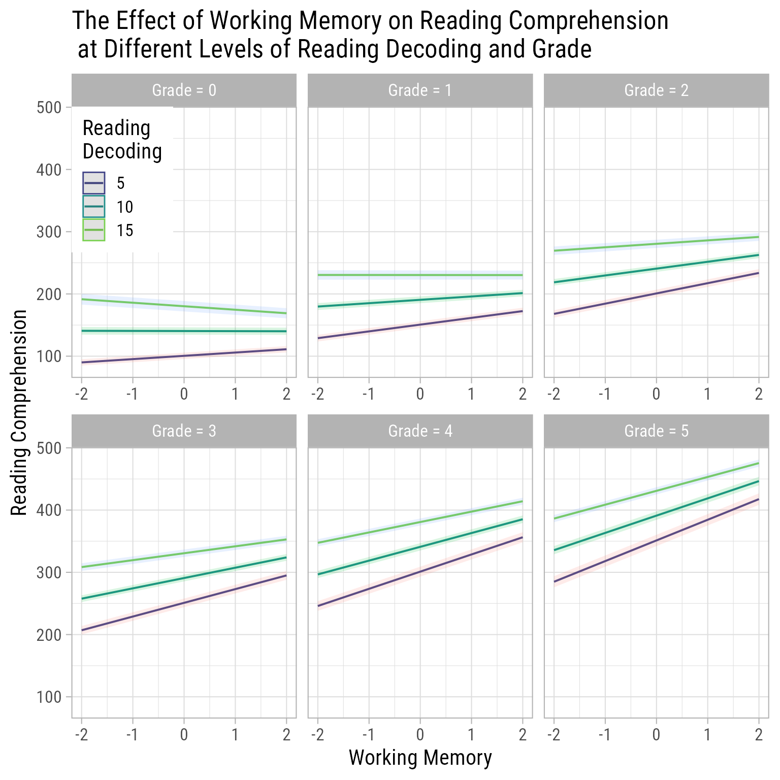
An alternate view of the same model suggests that the effect of working memory on reading comprehension is minimal in Kindergarten (Grade 0) and 1st grade when the focus is more on reading letters, single words, and very short sentences. However as the focus moves to longer, more complex sentences and paragraphs, the effect of Working Memory on Reading Comprehension increases.

plot_model(fit_final, 
           type = "pred", 
           terms = c("working_memory [-2, 2]", "reading_decoding [5, 10, 15]", "Grade [0:5]"),
           title = "The Effect of Working Memory on Reading Comprehension\n at Different Levels of Reading Decoding and Grade")

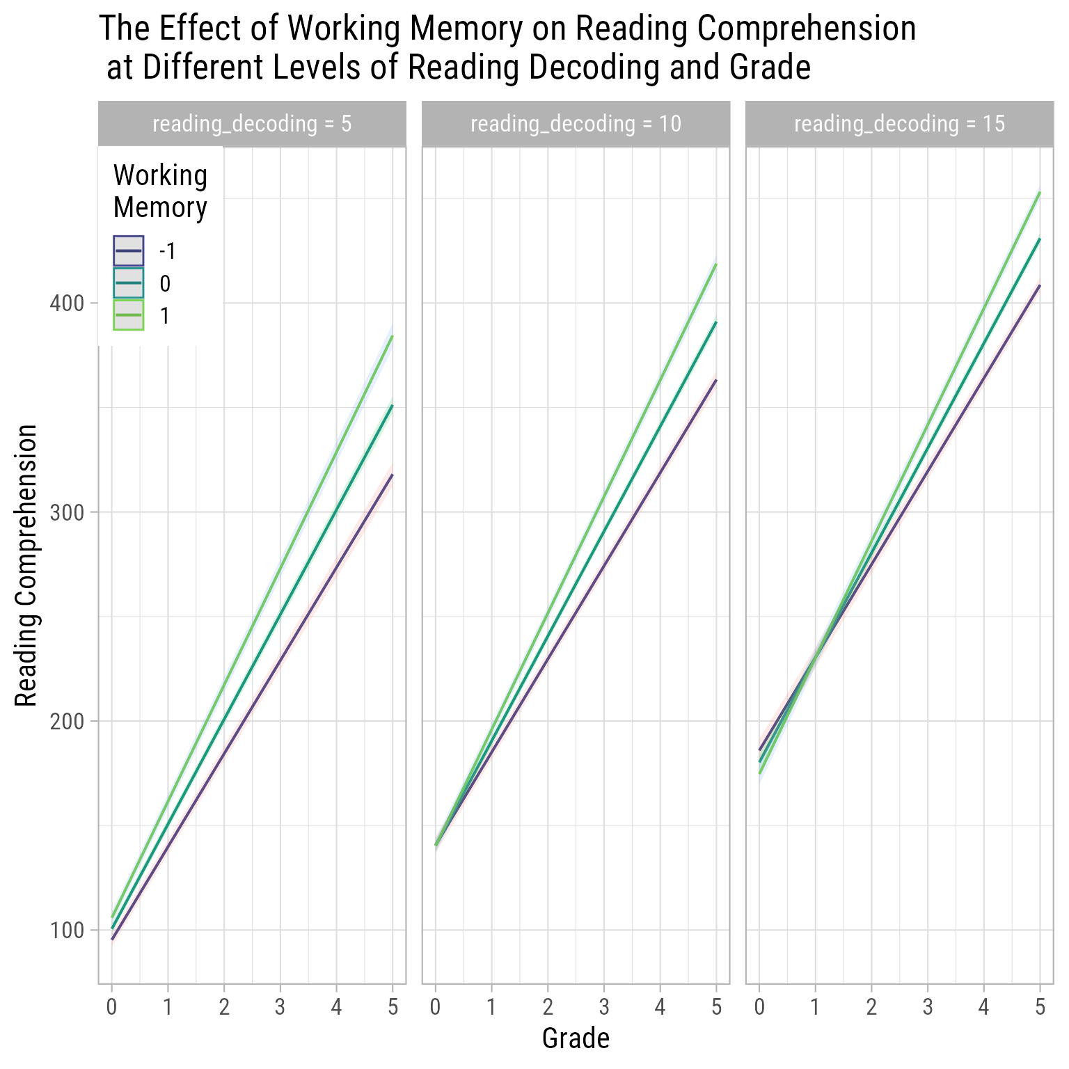
Another view of the same model suggests that students with higher Working Memory have faster Reading Comprehension growth rates, even after controlling for Reading Decoding.

plot_model(fit_final, 
           type = "pred", 
           terms = c("Grade [0:5]", "working_memory [-1, 0, 1]", "reading_decoding [5, 10, 15]"),
           title = "The Effect of Working Memory on Reading Comprehension\n at Different Levels of Reading Decoding and Grade") + 
  theme(legend.position = c(1,0), legend.justification = c(1,0))

Reflect

How this method could be used in your own research?

Exercise

Imagine that n = 1000 participants with anxiety disorders were in a 10-week study of meditation’s effect on reducing anxiety over time. Each participant was assigned to a student therapist who taught the meditation techniques to the participants. Transcriptions of the instruction session were rated for levels of therapist support.

Variables:

  • person_id: The identifier for each person
  • Week : The week on which data were collected, starting with Week 0 and ending on Week 4.
  • Anxiety: The overall level of Anxiety participants reported for the Week (level 1).
  • therapist_support A person-level (level 2) rating of overall therapist support.
  • minutes_meditating The total hours spent meditating each week.

Predictions:

  • The more time spent each week in meditation, the more anxiety will reduce over time. Note that this is NOT a prediction that the simple effect of meditation will be positive. It is instead a prediction that meditation will interact (negatively) with the time variable Week.
  • The therapist’s overall level of support is predicted to interact with time (i.e., Week) such that participants with more supportive therapists will improve more quickly than participants with less support therapists.
  • The therapist’s overall level of support is predicted to increase the potency of meditation’s effect over time. That is, a negative value is predicted for the 3-way interaction between therapist support, minutes meditated, and time (Week).

Load Data and Packages

library(tidyverse)
library(lme4)
library(easystats)
library(sjPlot)

d <- read_csv("https://github.com/wjschne/EDUC5529/raw/master/hw7_meditation.csv", 
              col_types = cols(
                person_id = col_factor(),
                Week = col_integer(),
                Anxiety = col_double(),
                meditation_hours = col_integer(),
                therapist_support = col_double())) 

Fit random intercept model

Try setting up the code yourself. Call the model fit_0

Run the summary function and the model_performance function on the model.

fit_0 <- lmer(Anxiety ~ 1 + (1 | person_id), data = d)
summary(fit_0)
performance::model_performance(fit_0)

Between-Person Proportion of Variance

Question 1

Where would you look in the output for summary(fit_0) to find the average level of Anxiety across the entire data set?

Question 2

In model fit_0, what proportion of variance in Anxiety is between persons?

Let’s make a nice table

sjPlot::tab_model(fit_0)
  Anxiety
Predictors Estimates CI p
(Intercept) 65.00 64.62 – 65.38 <0.001
Random Effects
σ2 69.71
τ00 person_id 30.32
ICC 0.30
N person_id 1000
Observations 11000
Marginal R2 / Conditional R2 0.000 / 0.303
Table 3: Null Model Results

Fit the linear effect of time (i.e., Week)

Estimate the linear effect of Week. Try setting up the code yourself. Call the model fit_week

Run summary, model_performance, and report on the model.

fit_week <- lmer(Anxiety ~ 1 + Week + (1 | person_id), data = d)
summary(fit_week)
performance::model_performance(fit_week)
report::report(fit_week)

Let’s compare the fit of both models:

anova(fit_0, fit_week)
Data: d
Models:
fit_0: Anxiety ~ 1 + (1 | person_id)
fit_week: Anxiety ~ 1 + Week + (1 | person_id)
         npar   AIC   BIC logLik deviance  Chisq Df Pr(>Chisq)    
fit_0       3 79664 79686 -39829    79658                         
fit_week    4 77765 77794 -38878    77757 1901.6  1  < 2.2e-16 ***
---
Signif. codes:  0 '***' 0.001 '**' 0.01 '*' 0.05 '.' 0.1 ' ' 1
compare_performance(fit_0, fit_week)
# Comparison of Model Performance Indices

Name     |   Model |   AIC (weights) |  AICc (weights) |   BIC (weights)
------------------------------------------------------------------------
fit_0    | lmerMod | 79664.4 (<.001) | 79664.4 (<.001) | 79686.3 (<.001)
fit_week | lmerMod | 77764.8 (>.999) | 77764.8 (>.999) | 77794.0 (>.999)

Name     | R2 (cond.) | R2 (marg.) |   ICC |  RMSE | Sigma
----------------------------------------------------------
fit_0    |      0.303 |      0.000 | 0.303 | 8.029 | 8.349
fit_week |      0.424 |      0.110 | 0.353 | 7.290 | 7.592

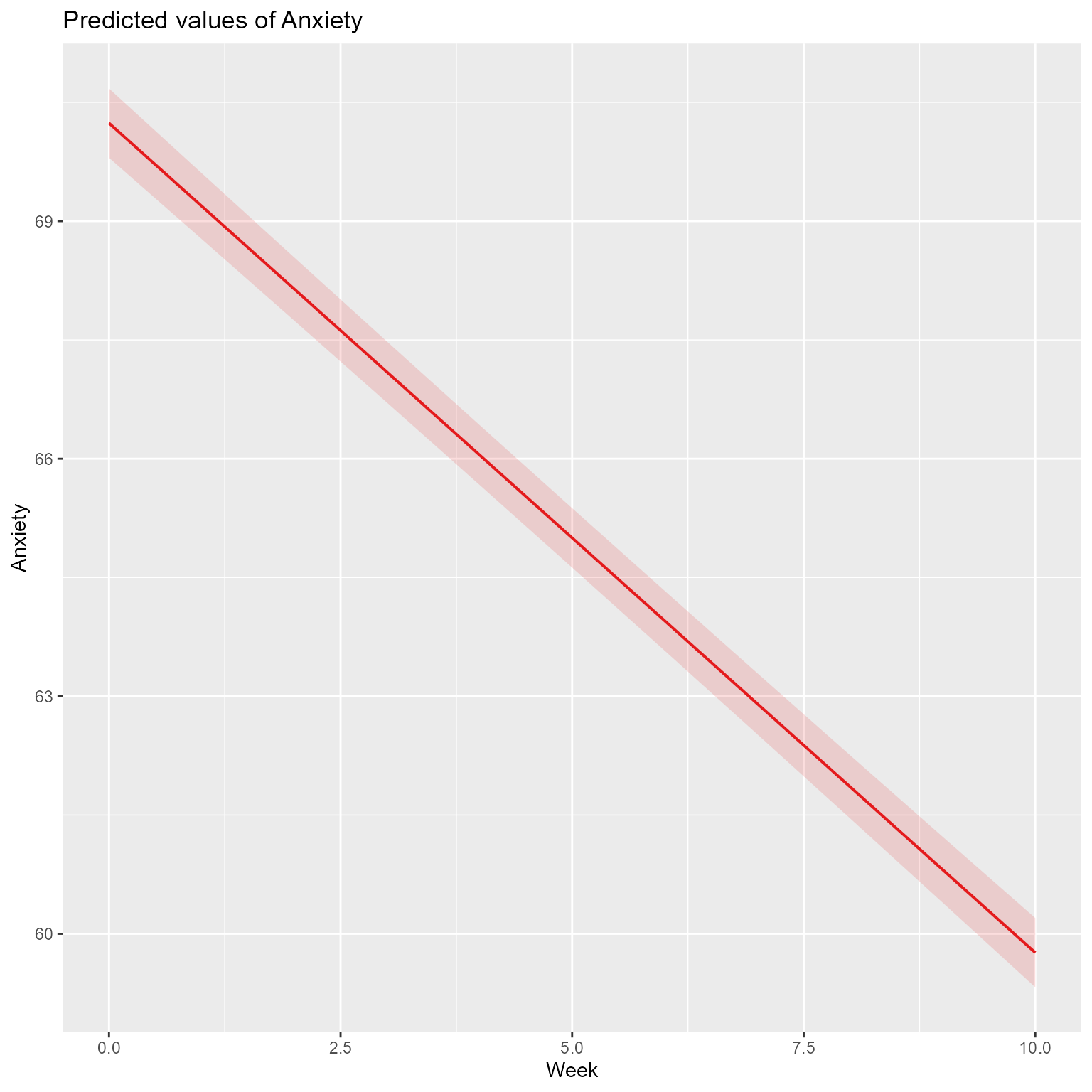
By every criterion, fit_week fits better than fit_0. Thus, there is a significant association with Week and Anxiety. Because the slope of Week is negative, people’s anxiety decreased over time by about -1.05 points per week.

Question 3

In model fit_week, what proportion of variance in Anxiety is explained by Week?

Look at the R2_marginal column in the performance::model_performance(fit_week) output.

Question 4

In the output of summary(fit_week), where would you look to see how much anxiety is changing from week to week, on average?

Plot the Model and Make a Nice Table

plot_model(fit_week, type = "pred", terms = "Week")
Figure 9: Predicted Effects of Week
tab_model(fit_0, fit_week, dv.labels = c("Null Model", "Week"), show.ci = F)
  Null Model Week
Predictors Estimates p Estimates p
(Intercept) 65.00 <0.001 70.24 <0.001
Week -1.05 <0.001
Random Effects
σ2 69.71 57.64
τ00 30.32 person_id 31.42 person_id
ICC 0.30 0.35
N 1000 person_id 1000 person_id
Observations 11000 11000
Marginal R2 / Conditional R2 0.000 / 0.303 0.110 / 0.424
Table 4: The Linear Effect of Week

Add the quadratic effect of Week.

We did not predict non-linear effects of time, but it is good idea to check. Usually you include enough polynomial degrees to be consistent with your models. If you have no prediction, add them one at a time, but be conservative in doing so.

fit_week_2 <- lmer(Anxiety ~ 1 + poly(Week, 2) + (1 | person_id), data = d)
summary(fit_week_2)
Linear mixed model fit by REML ['lmerMod']
Formula: Anxiety ~ 1 + poly(Week, 2) + (1 | person_id)
   Data: d

REML criterion at convergence: 77745.6

Scaled residuals: 
    Min      1Q  Median      3Q     Max 
-6.9612 -0.4497  0.1040  0.6023  2.8793 

Random effects:
 Groups    Name        Variance Std.Dev.
 person_id (Intercept) 31.42    5.605   
 Residual              57.64    7.592   
Number of obs: 11000, groups:  person_id, 1000

Fixed effects:
                Estimate Std. Error t value
(Intercept)      65.0000     0.1915 339.502
poly(Week, 2)1 -347.4464     7.5924 -45.763
poly(Week, 2)2   -6.9694     7.5924  -0.918

Correlation of Fixed Effects:
            (Intr) p(W,2)1
poly(Wk,2)1 0.000         
poly(Wk,2)2 0.000  0.000  
anova(fit_week, fit_week_2)
Data: d
Models:
fit_week: Anxiety ~ 1 + Week + (1 | person_id)
fit_week_2: Anxiety ~ 1 + poly(Week, 2) + (1 | person_id)
           npar   AIC   BIC logLik deviance  Chisq Df Pr(>Chisq)
fit_week      4 77765 77794 -38878    77757                     
fit_week_2    5 77766 77802 -38878    77756 0.8428  1     0.3586

Here we see that the quadratic effect of Week is not significant, so we need not continue adding polynomial degrees. If we did, it would look like this:

fit_week_3 <- lmer(Anxiety ~ 1 + poly(Week, 3) + (1 | person_id), data = d)
summary(fit_week_3)
Linear mixed model fit by REML ['lmerMod']
Formula: Anxiety ~ 1 + poly(Week, 3) + (1 | person_id)
   Data: d

REML criterion at convergence: 77737.9

Scaled residuals: 
    Min      1Q  Median      3Q     Max 
-6.9654 -0.4497  0.1032  0.6000  2.8946 

Random effects:
 Groups    Name        Variance Std.Dev.
 person_id (Intercept) 31.42    5.605   
 Residual              57.64    7.592   
Number of obs: 11000, groups:  person_id, 1000

Fixed effects:
                Estimate Std. Error t value
(Intercept)      65.0000     0.1915 339.502
poly(Week, 3)1 -347.4464     7.5920 -45.765
poly(Week, 3)2   -6.9694     7.5920  -0.918
poly(Week, 3)3  -10.3752     7.5920  -1.367

Correlation of Fixed Effects:
            (Intr) p(W,3)1 p(W,3)2
poly(Wk,3)1 0.000                 
poly(Wk,3)2 0.000  0.000          
poly(Wk,3)3 0.000  0.000   0.000  
anova(fit_week, fit_week_2, fit_week_3)
Data: d
Models:
fit_week: Anxiety ~ 1 + Week + (1 | person_id)
fit_week_2: Anxiety ~ 1 + poly(Week, 2) + (1 | person_id)
fit_week_3: Anxiety ~ 1 + poly(Week, 3) + (1 | person_id)
           npar   AIC   BIC logLik deviance  Chisq Df Pr(>Chisq)
fit_week      4 77765 77794 -38878    77757                     
fit_week_2    5 77766 77802 -38878    77756 0.8428  1     0.3586
fit_week_3    6 77766 77810 -38877    77754 1.8679  1     0.1717

Given the lack of polynomial effects, we will stick with just the linear effect in fit_week.

Add the L1 time-covarying predictor, meditation_hours to the model

Try setting up the code yourself. Call the model fit_meditation

Run summary, model_performance, and report on the model. Compare fit_meditation with the previous model, fit_week.

fit_meditation <- lmer(Anxiety ~ 1 + Week + meditation_hours + (1 | person_id), data = d)
summary(fit_meditation)
performance::model_performance(fit_meditation)
report::report(fit_meditation)

anova(fit_week, fit_meditation)
compare_performance(fit_week, fit_meditation)

When you the output, you will see that the effect of meditation_hours is significant. From the report function, the standardized beta (the effect if all variables were standardized) for meditation_hours is larger than the effect of Week. Theoretically, this result makes sense. Anxiety should decrease because of the intervention, not just because of time passing. Still, the effect of Week is significant, perhaps because of therapist contact and/or regression to the mean.

Nice plot and table:
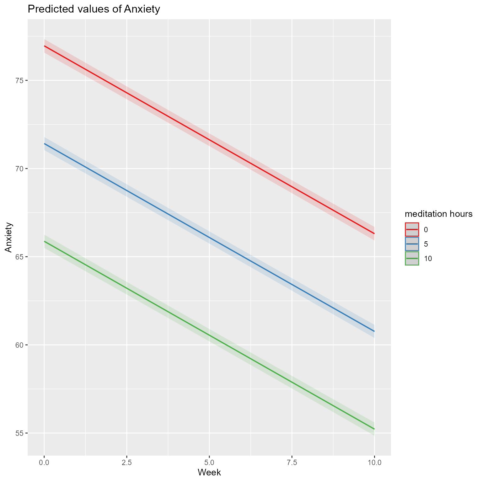
plot_model(fit_meditation, 
           type = "pred", 
           terms = c("Week", "meditation_hours [0, 5, 10]"))
Figure 10: The Predicted Effects of Week by Meditation Hours
tab_model(fit_meditation)
  Anxiety
Predictors Estimates CI p
(Intercept) 76.96 76.57 – 77.34 <0.001
Week -1.07 -1.09 – -1.04 <0.001
meditation hours -1.11 -1.12 – -1.09 <0.001
Random Effects
σ2 20.60
τ00 person_id 29.20
ICC 0.59
N person_id 1000
Observations 11000
Marginal R2 / Conditional R2 0.497 / 0.792
Table 5: Model for the Combined Effects of Week and Meditation

Add the predicted interaction of Week and meditation_hours.

Call the model fit_week_x_meditation

fit_week_x_meditation <- lmer(Anxiety ~ 1 + Week * meditation_hours + (1 | person_id), data = d)
summary(fit_week_x_meditation)
Linear mixed model fit by REML ['lmerMod']
Formula: Anxiety ~ 1 + Week * meditation_hours + (1 | person_id)
   Data: d

REML criterion at convergence: 61358.3

Scaled residuals: 
    Min      1Q  Median      3Q     Max 
-4.0746 -0.6355  0.0015  0.6369  4.4524 

Random effects:
 Groups    Name        Variance Std.Dev.
 person_id (Intercept) 29.50    5.431   
 Residual              11.36    3.370   
Number of obs: 11000, groups:  person_id, 1000

Fixed effects:
                       Estimate Std. Error t value
(Intercept)           71.866534   0.194086 370.281
Week                  -0.041797   0.015228  -2.745
meditation_hours      -0.267135   0.011141 -23.978
Week:meditation_hours -0.170020   0.001884 -90.265

Correlation of Fixed Effects:
            (Intr) Week   mdttn_
Week        -0.392              
medittn_hrs -0.348  0.626       
Wk:mdttn_hr  0.290 -0.745 -0.836
performance::model_performance(fit_week_x_meditation)
# Indices of model performance

AIC       |      AICc |       BIC | R2 (cond.) | R2 (marg.) |   ICC |  RMSE | Sigma
-----------------------------------------------------------------------------------
61370.252 | 61370.260 | 61414.086 |      0.885 |      0.588 | 0.722 | 3.219 | 3.370
report::report(fit_week_x_meditation)
We fitted a linear mixed model (estimated using REML and nloptwrap optimizer)
to predict Anxiety with Week and meditation_hours (formula: Anxiety ~ 1 + Week
* meditation_hours). The model included person_id as random effect (formula: ~1
| person_id). The model's total explanatory power is substantial (conditional
R2 = 0.89) and the part related to the fixed effects alone (marginal R2) is of
0.59. The model's intercept, corresponding to Week = 0 and meditation_hours =
0, is at 71.87 (95% CI [71.49, 72.25], t(10994) = 370.28, p < .001). Within
this model:

  - The effect of Week is statistically significant and negative (beta = -0.04,
95% CI [-0.07, -0.01], t(10994) = -2.74, p = 0.006; Std. beta = -0.33, 95% CI
[-0.34, -0.33])
  - The effect of meditation hours is statistically significant and negative
(beta = -0.27, 95% CI [-0.29, -0.25], t(10994) = -23.98, p < .001; Std. beta =
-0.62, 95% CI [-0.63, -0.62])
  - The effect of Week × meditation hours is statistically significant and
negative (beta = -0.17, 95% CI [-0.17, -0.17], t(10994) = -90.26, p < .001;
Std. beta = -0.30, 95% CI [-0.31, -0.29])

Standardized parameters were obtained by fitting the model on a standardized
version of the dataset. 95% Confidence Intervals (CIs) and p-values were
computed using a Wald t-distribution approximation.
anova(fit_meditation, fit_week_x_meditation)
Data: d
Models:
fit_meditation: Anxiety ~ 1 + Week + meditation_hours + (1 | person_id)
fit_week_x_meditation: Anxiety ~ 1 + Week * meditation_hours + (1 | person_id)
                      npar   AIC   BIC logLik deviance  Chisq Df Pr(>Chisq)    
fit_meditation           5 67309 67345 -33649    67299                         
fit_week_x_meditation    6 61342 61386 -30665    61330 5968.7  1  < 2.2e-16 ***
---
Signif. codes:  0 '***' 0.001 '**' 0.01 '*' 0.05 '.' 0.1 ' ' 1
compare_performance(fit_meditation, fit_week_x_meditation)
# Comparison of Model Performance Indices

Name                  |   Model |   AIC (weights) |  AICc (weights)
-------------------------------------------------------------------
fit_meditation        | lmerMod | 67308.9 (<.001) | 67308.9 (<.001)
fit_week_x_meditation | lmerMod | 61342.2 (>.999) | 61342.2 (>.999)

Name                  |   BIC (weights) | R2 (cond.) | R2 (marg.) |   ICC
-------------------------------------------------------------------------
fit_meditation        | 67345.4 (<.001) |      0.792 |      0.497 | 0.586
fit_week_x_meditation | 61386.0 (>.999) |      0.885 |      0.588 | 0.722

Name                  |  RMSE | Sigma
-------------------------------------
fit_meditation        | 4.340 | 4.538
fit_week_x_meditation | 3.219 | 3.370
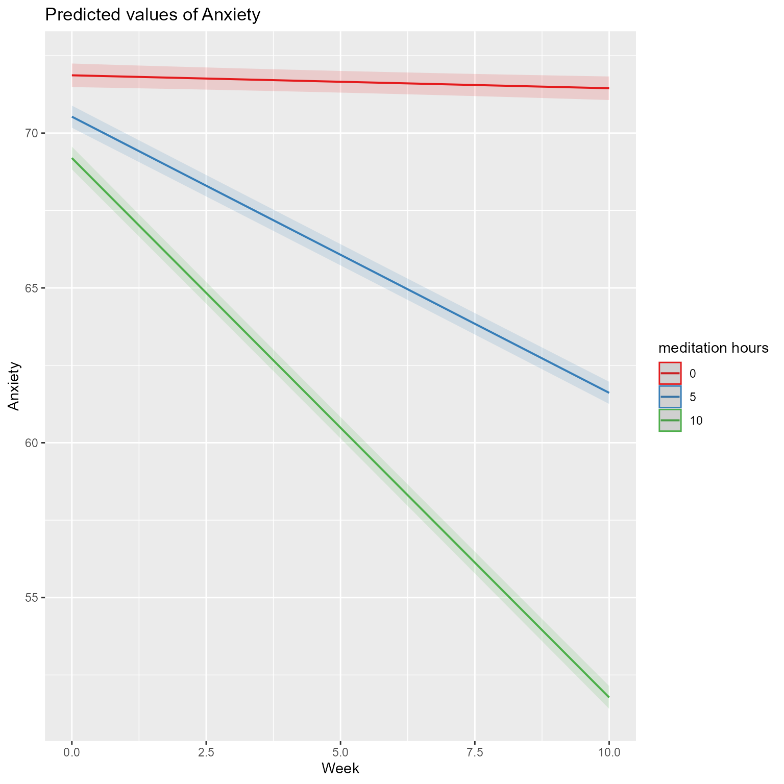
plot_model(fit_week_x_meditation, type = "pred", terms = c("Week", "meditation_hours [0, 5, 10]"))

tab_model(fit_week_x_meditation)
  Anxiety
Predictors Estimates CI p
(Intercept) 71.87 71.49 – 72.25 <0.001
Week -0.04 -0.07 – -0.01 0.006
meditation hours -0.27 -0.29 – -0.25 <0.001
Week × meditation hours -0.17 -0.17 – -0.17 <0.001
Random Effects
σ2 11.36
τ00 person_id 29.50
ICC 0.72
N person_id 1000
Observations 11000
Marginal R2 / Conditional R2 0.588 / 0.885

We see that the hypothesized interaction is significant, meaning that the effect of Week depends on meditation_hours. In the plot, you can see that the reduction of Anxiety over time is larger for people who meditation more.

Note that in the output the fixed effects of Week and meditation_hours are simple slopes. They tell us what the slope of the variable is when the other predictors in the interaction are 0. For statistical significance of simple slopes, you can look in the output of report.

Question 5

In model fit_week_x_meditation, when meditation_hours is 0, is the slope of Week statistically significant?

Add the L2 predictor

Add therapist_support to the previous model. Call the model fit_support. Run summary, model_performance, and report on the model. Compare fit_support with the previous model, fit_meditation.

Set up the Code

Try setting up the code yourself.

fit_support <- lmer(Anxiety ~ Week * meditation_hours + therapist_support + (1 | person_id), data = d)
summary(fit_support)
performance::model_performance(fit_support)
report::report(fit_support)

anova(fit_meditation, fit_support)
compare_performance(fit_meditation, fit_support, rank = T)

After running the code, you can see that the therapist support is associated with lower levels of anxiety.

Add random slopes for Level 1 predictors.

In general, be conservative about adding random slopes to your model. They often cause convergence problems and long computation times.

Let’s see if we need Week to have a random slope.

fit_week_random <- lmer(Anxiety ~ Week * meditation_hours + therapist_support + (1 + Week || person_id), data = d)
summary(fit_week_random)
Linear mixed model fit by REML ['lmerMod']
Formula: Anxiety ~ Week * meditation_hours + therapist_support + ((1 |  
    person_id) + (0 + Week | person_id))
   Data: d

REML criterion at convergence: 61325.2

Scaled residuals: 
    Min      1Q  Median      3Q     Max 
-4.0529 -0.6342  0.0016  0.6357  4.4314 

Random effects:
 Groups      Name        Variance  Std.Dev.
 person_id   (Intercept) 28.414902 5.33056 
 person_id.1 Week         0.005105 0.07145 
 Residual                11.303273 3.36203 
Number of obs: 11000, groups:  person_id, 1000

Fixed effects:
                       Estimate Std. Error t value
(Intercept)           71.847112   0.191278 375.616
Week                  -0.041067   0.015396  -2.667
meditation_hours      -0.265533   0.011158 -23.797
therapist_support     -1.011291   0.173201  -5.839
Week:meditation_hours -0.170138   0.001888 -90.134

Correlation of Fixed Effects:
            (Intr) Week   mdttn_ thrps_
Week        -0.394                     
medittn_hrs -0.354  0.621              
thrpst_sppr  0.016 -0.004 -0.022       
Wk:mdttn_hr  0.295 -0.738 -0.836  0.004
performance::model_performance(fit_week_random)
# Indices of model performance

AIC       |      AICc |       BIC | R2 (cond.) | R2 (marg.) |   ICC |  RMSE | Sigma
-----------------------------------------------------------------------------------
61341.222 | 61341.235 | 61399.668 |      0.888 |      0.607 | 0.715 | 3.203 | 3.362
anova(fit_support, fit_week_random, refit = FALSE)
Data: d
Models:
fit_support: Anxiety ~ Week * meditation_hours + therapist_support + (1 | person_id)
fit_week_random: Anxiety ~ Week * meditation_hours + therapist_support + ((1 | person_id) + (0 + Week | person_id))
                npar   AIC   BIC logLik deviance  Chisq Df Pr(>Chisq)
fit_support        7 61340 61392 -30663    61326                     
fit_week_random    8 61341 61400 -30663    61325 1.2712  1     0.2595

There is not a significant effect here. Note the use of refit = FALSE in the anova function. This is good practice when comparing models that differ only in their random effects.

fit_meditation_random <- lmer(Anxiety ~ Week * meditation_hours + therapist_support + (1 + meditation_hours || person_id), data = d)
summary(fit_meditation_random)
Linear mixed model fit by REML ['lmerMod']
Formula: Anxiety ~ Week * meditation_hours + therapist_support + ((1 |  
    person_id) + (0 + meditation_hours | person_id))
   Data: d

REML criterion at convergence: 61323.8

Scaled residuals: 
    Min      1Q  Median      3Q     Max 
-4.0732 -0.6349  0.0008  0.6351  4.4356 

Random effects:
 Groups      Name             Variance  Std.Dev.
 person_id   (Intercept)      28.580662 5.34609 
 person_id.1 meditation_hours  0.002205 0.04696 
 Residual                     11.287908 3.35975 
Number of obs: 11000, groups:  person_id, 1000

Fixed effects:
                       Estimate Std. Error t value
(Intercept)           71.847721   0.191808 374.581
Week                  -0.041972   0.015251  -2.752
meditation_hours      -0.265514   0.011376 -23.339
therapist_support     -0.999116   0.173555  -5.757
Week:meditation_hours -0.169966   0.001904 -89.250

Correlation of Fixed Effects:
            (Intr) Week   mdttn_ thrps_
Week        -0.398                     
medittn_hrs -0.350  0.621              
thrpst_sppr  0.016 -0.002 -0.019       
Wk:mdttn_hr  0.295 -0.746 -0.829  0.002
optimizer (nloptwrap) convergence code: 0 (OK)
Model failed to converge with max|grad| = 0.00610441 (tol = 0.002, component 1)
performance::model_performance(fit_meditation_random)
# Indices of model performance

AIC       |      AICc |       BIC | R2 (cond.) | R2 (marg.) |   ICC |  RMSE | Sigma
-----------------------------------------------------------------------------------
61339.774 | 61339.787 | 61398.220 |      0.888 |      0.605 | 0.717 | 3.200 | 3.360
anova(fit_support, fit_meditation_random, refit = FALSE)
Data: d
Models:
fit_support: Anxiety ~ Week * meditation_hours + therapist_support + (1 | person_id)
fit_meditation_random: Anxiety ~ Week * meditation_hours + therapist_support + ((1 | person_id) + (0 + meditation_hours | person_id))
                      npar   AIC   BIC logLik deviance  Chisq Df Pr(>Chisq)  
fit_support              7 61340 61392 -30663    61326                       
fit_meditation_random    8 61340 61398 -30662    61324 2.7192  1    0.09915 .
---
Signif. codes:  0 '***' 0.001 '**' 0.01 '*' 0.05 '.' 0.1 ' ' 1

Again, no significant effect here. We are not really sure, however, because the model did not converge. However, we did not predict a random slope, so to be conservative, we revert back to fit_support as our comparison model.

Add hypothesized interaction terms

We hypothesized a 3-way interaction of Week, meditation_hours, and therapist_support. Add it to the fit_support model.

Try setting up the code yourself. Call the model fit_3_way_interaction.

Pretend that the warning (boundary (singular) fit: see ?isSingular) is not there.

Run summary, model_performance, and report on the model.

fit_3_way_interaction <- lmer(Anxiety ~ Week * meditation_hours * therapist_support + (1 | person_id), data = d)
summary(fit_3_way_interaction)
performance::model_performance(fit_3_way_interaction)
report::report(fit_3_way_interaction)

Let’s compare the fit of both models:

anova(fit_support, fit_3_way_interaction)
Data: d
Models:
fit_support: Anxiety ~ Week * meditation_hours + therapist_support + (1 | person_id)
fit_3_way_interaction: Anxiety ~ Week * meditation_hours * therapist_support + (1 | person_id)
                      npar   AIC   BIC logLik deviance  Chisq Df Pr(>Chisq)    
fit_support              7 61311 61362 -30648    61297                         
fit_3_way_interaction   10 61296 61369 -30638    61276 20.502  3  0.0001336 ***
---
Signif. codes:  0 '***' 0.001 '**' 0.01 '*' 0.05 '.' 0.1 ' ' 1
compare_performance(fit_support, fit_3_way_interaction, rank = T)
# Comparison of Model Performance Indices

Name                  |   Model | R2 (cond.) | R2 (marg.) |   ICC |  RMSE
-------------------------------------------------------------------------
fit_3_way_interaction | lmerMod |      0.888 |      0.606 | 0.715 | 3.216
fit_support           | lmerMod |      0.888 |      0.605 | 0.715 | 3.219

Name                  | Sigma | AIC weights | AICc weights | BIC weights | Performance-Score
--------------------------------------------------------------------------------------------
fit_3_way_interaction | 3.368 |       0.999 |        0.999 |       0.024 |            87.50%
fit_support           | 3.370 |    7.09e-04 |     7.12e-04 |       0.976 |            12.50%

The results of the anova model comparison is significant, but we can see that the three-way interaction is not. Let’s plot the model and see what is going on.
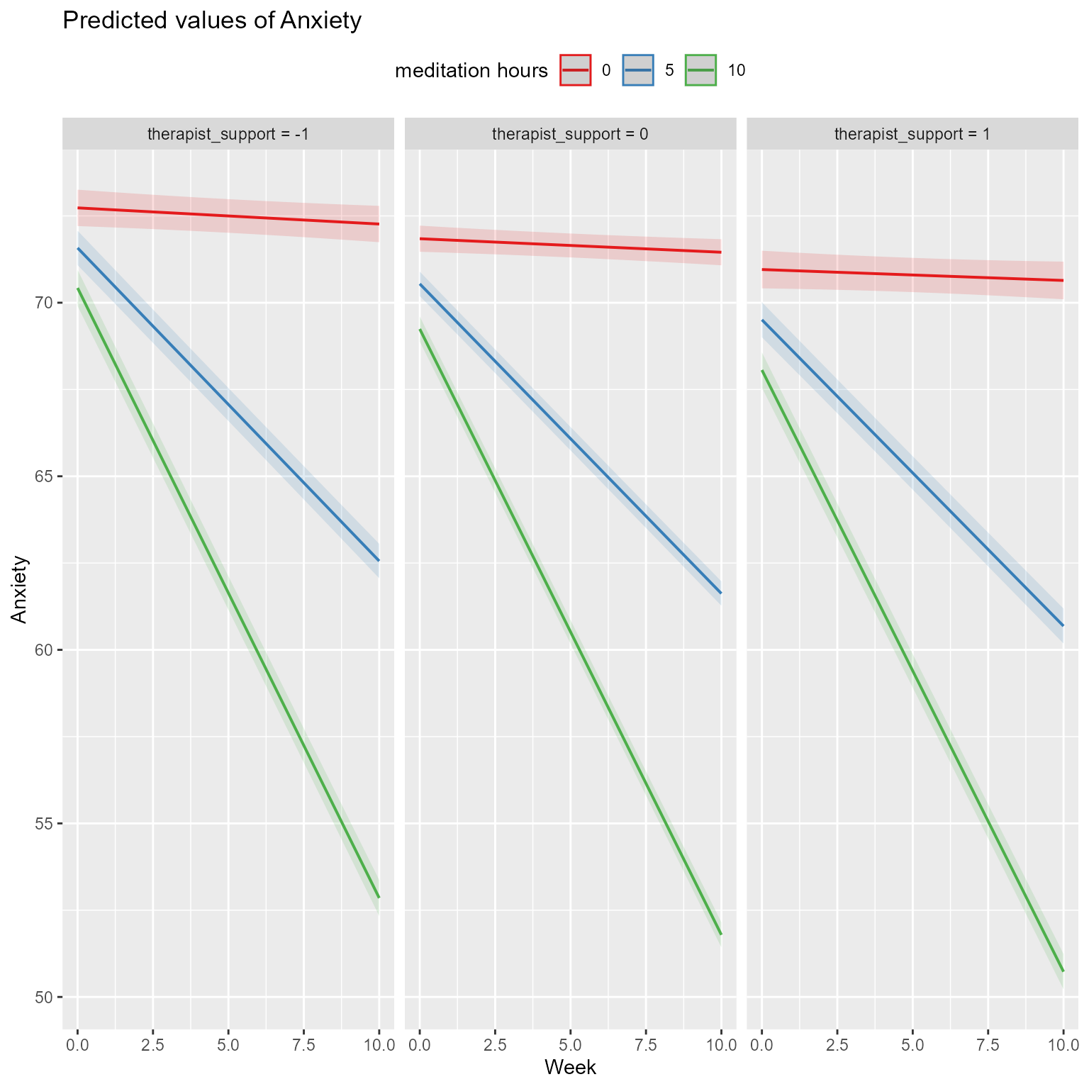
plot_model(fit_3_way_interaction, 
           type = "pred", 
           terms = c("Week", "meditation_hours [0, 5, 10]", "therapist_support [-1, 0, 1]")) + 
  theme(legend.position = "top")
Figure 11: Interaction of Week, Meditation, and Therapist Support

From the plot and the summary output, the significant effect appears to be in the 2-way interaction of meditation_hours and therapist_support. You cannot be sure about that until you run the model.

Add 2-way interaction

Add the interaction of therapist_support and meditation_hoursto the fit_support model

Try setting up the code yourself. Call the model fit_support_x_meditation.

Run summary, model_performance, and report on the model.

fit_support_x_meditation <- lmer(Anxiety ~ Week * meditation_hours + meditation_hours * therapist_support + (1 | person_id), data = d)

summary(fit_support_x_meditation)

performance::model_performance(fit_support_x_meditation)
report::report(fit_support_x_meditation)
Question 6

In the fit_support_x_meditation model, is the interaction of meditation_hours and therapist_support significant?