Major Steps for Power Analysis Via Simulation

Specify Model
Create a Data Generator Function that Creates a Single Data Set
Create a Model Fitting Function
Create a Detect Effect Function
Generate Many Data Sets with Varying Sample Sizes
Test the Model on Each Data Set
Plot the Relation Between Sample Size and the Probability of Detecting the Effect.

Our Study’s Rationale

When a student persistently fails to learn to read (or write or calculate or …), we generally want to do something different so that the child’s learning trajectory changes. Traditionally, school psychologists conducted comprehensive psychoeducational assessments to find out what was holding the student back and then specify recommended interventions. These assessments included measures of cognitive abilities, personality, psychopathology, and academic skills. It involved interviewing students, parents, and teachers as well as direct observations in the classroom. Unfortunately, such assessments are costly in terms of time, resources, and personnel. Furthermore, it has always been assumed that a comprehensive assessment is useful, but the treatment utility of assessment has not generally be demonstrated.

Instead of performing a comprehensive assessment, one can simply measure whether a student is behind academically and administer empirically-validated interventions designed to remediate any academic skill deficits. This approach is efficient and works well for most students. However, there is a smaller group of students for whom this approach results in repeated failure to respond to intervention.

What should we do with students who repeatedly fail to respond to intervention. One option is to select a different empirically-validated intervention and try again. Sometimes this will work, and sometimes another treatment failure will occur. A second option is to try a comprehensive assessment to figure out what is going on. If comprehensive assessments are helpful, we should see a higher likelihood of treatment response after the assessment.

Study Design

To make this tutorial easier to follow, I am going to make my assumptions much simpler than I would if I were planning a real study. Please know that I understand that student learning is much more complicated than the study I propose here.

Our task is to design an experiment that would reveal whether comprehensive assessments have any effect on student learning. We would like to plan our study so that we are likely to find the effect of comprehensive assessments if it exists, but also conserve resources by making the study as small and as short as we can.

Let’s say that the learning domain is reading comprehension. Let’s assume that every month students are given an assessment of their reading comprehension ability. On average, most students make one month of progress each assessment. However, we have a sample of children who are not making adequate progress. Every month, they are making about .25 months of progress. So their growth rate, on average is .25, and we expect a growth rate of 1.

To qualify for the student, the students must have 4 months of slow progress. Thus, we will have data for 4 months prior to the assessment.

Specify Model

Level 1: Measurement Occasion

Although the model can appear complicated, the idea here is simple: At first reading grows slowly each month. Once an assessment has occurred, the reading growth rate is faster.

\begin{align*} Reading_{ti} &= b_{0i}+b_{1i}Month_{ti}+b_{2i}MonthsAfterAssessment_{ti}+e_{ti}\\ e_{ti}&\sim\mathcal{N}(0, \sigma_e^2) \end{align*}

Variable	Interpretation
Reading_{ti}	The measure of Reading Comprehension for person i at month t.
b_{0i}	The predicted level of Reading Comprehension for person i at month 0.
Month_{ti}	The number of months elapsed for person i at month t.
b_{1i}	The pre-assessment growth rate in reading comprehension for person i at month t.
MonthsAfterAssessment_{ti}	The number of months after the assessment for person i at month t.
b_{2i}	The degree to which assessment increases growth rate in reading comprehension for person i at month t.
e_{ti}	The deviation from expectations for Reading Comprehension at occasion t for person i. It represents the model’s failure to accurately predict Reading Comprehension at each measurement occasion.
\sigma_e^2	The variance of e_{ti}

Level 2: Student

For the sake of simplicity, the model does not include any student-level predictors.

\begin{align*} b_{0i} &= b_{00}+e_{0i}\\ b_{1i} &= b_{10}+e_{1i}\\ b_{2i} &= b_{20}\\ \boldsymbol{e}_2 &= \begin{bmatrix}e_{0i}\\e_{1i}\end{bmatrix}\\ \boldsymbol{e}_2&\sim\mathcal{N}\left(\boldsymbol{0},\boldsymbol{\tau}\right)\\ \boldsymbol{\tau} &= \begin{bmatrix}\tau_{00} & \tau_{10} \\ \tau_{10} & \tau_{11}\end{bmatrix} \end{align*}

Variable	Interpretation
b_{0i}	The predicted level of Reading Comprehension for person i at month 0.
b_{00}	The overall predicted value of Reading Comprehension at month 0.
e_{0i}	Person i’s deviation from expectations for the random intercept. It represents the model’s failure to predict each person’s random intercept.
b_{1i}	The pre-assessment growth rate in reading comprehension for person i at month t.
b_{10}	The rate at which Reading Comprehension increases for each month if no assessment has occurred (i.e., when MonthsAfterAssessment_{ti} = 0).
e_{1i}	Person i’s the deviation from expectations for the random slope for month. It represents the model’s failure to predict each person’s rate of increase in Reading Comprehension over time (after controlling for months after assessment).
b_{2i}	The degree to which assessment increases growth rate in reading comprehension for person i at month t. Because no random component is included, it equals b_{20}.
b_{20}	The overall degree to which assessment increases growth rate in reading comprehension.
\boldsymbol{e}_2	The 1-column matrix of Level-2 random effects (i.e., e_{0i} and e_{1i})
\boldsymbol{\tau}	The covariance matrix of of Level-2 random effects
\tau_{00}	The variance of e_{0i}
\tau_{11}	The variance of e_{1i}
\tau_{10}	The covariance of e_{0i} and e_{1i}

Hypothesized Model as a `lmer` formula

reading ~ 1 + month + months_after_assessment + (1 + month | student_id)

Data Generator Function

There are many ways to do this. Often people separate their power analysis simulations into many functions, but here I am going to make one function that creates data, one that performs the analysis, and one that returns TRUE if the effect is significant (in this case, t > 2).

# Load packages
library(tidyverse)
library(mvtnorm)
library(lme4)
library(lavaan)
library(broom)


make_data <- function(
  n = 100, # Sample size (number of students)
  # Fixed effects
  b_00, # fixed intercept
  b_10, # fixed slope for month
  b_20, # fixed slope for moths after assessment
  # Level-2 random effects covariance matrix
  tau_00, # variance of random intercept
  tau_11, # variance of slope for month
  r_01, # correlation between random intercept and slope
  sigma_e = 2, # Level-1 random effect standard deviation
  k_months_total = 24, # Total months of study
  k_months_before = 4, # Months before study
  k_months_delay = 2 # Average delay before assessment
  ) {
  
  tau <- matrix(c(tau_00, tau_00 * tau_11 * r_01,
                  tau_00 * tau_11 * r_01, tau_11), 
                nrow = 2)
  
  # Level-2 random effects
  e_2 <- mvtnorm::rmvnorm(n, mean = c(e_0i = 0, e_1i = 0), sigma = tau) %>% 
  as_tibble()
  
  # Student-level data (Level 2)
  d_2 <- tibble(student_id = 1:n) %>%
    bind_cols(e_2) %>%
    mutate(
      b_0i = b_00 + e_0i,
      b_1i = b_10 + e_1i,
      b_2i = b_20,
      assessment_month = k_months_before + rpois(n, lambda = k_months_delay),
      k_months_total = k_months_total
    )
  
  # Occasion-level data (Level 1)
  d_1 <- d_2 %>%
    uncount(k_months_total) %>% # make copies of each row
    mutate(month = row_number() - 1, .by = student_id) %>% # Make months by group row number 
    mutate(
      months_after_assessment = ifelse(month < assessment_month,
                                       0,
                                       month - assessment_month),
      e_ij = rnorm(nrow(.), 0, sigma_e),
      reading = b_0i + b_1i * month + b_2i * months_after_assessment + e_ij
    )
}

Let’s generate one data set, perform the analysis, and plot it to see if it does what we what.

# Fixed effects
b_00 = 0 # Reading level at month 0
b_10 = 0.5 # Pre-assessment growth rate
b_20 = 0.5 # Assessment effect on growth rate


# Level-2 random effects covariance matrix
tau_00 = 16
tau_11 = 0.16
r_01 = 0


d <- make_data(n = 500, 
               b_00 = b_00, 
               b_10 = b_10, 
               b_20 = b_20, 
               tau_00 = tau_00,
               tau_11 = tau_11,
               r_01 = r_01,
               k_months_total = 24,
               k_months_before = 8,
               k_months_delay = 2)

fit <- lmer(reading ~ month + months_after_assessment + (month | student_id),
            data = d)

summary(fit)

Linear mixed model fit by REML ['lmerMod']
Formula: reading ~ month + months_after_assessment + (month | student_id)
   Data: d

REML criterion at convergence: 55121

Scaled residuals: 
   Min     1Q Median     3Q    Max 
-3.646 -0.658  0.004  0.642  4.667 

Random effects:
 Groups     Name        Variance Std.Dev. Corr 
 student_id (Intercept) 14.780   3.844         
            month        0.171   0.414    -0.09
 Residual                4.074   2.018         
Number of obs: 12000, groups:  student_id, 500

Fixed effects:
                        Estimate Std. Error t value
(Intercept)              -0.0511     0.1787   -0.29
month                     0.5221     0.0198   26.32
months_after_assessment   0.4914     0.0111   44.30

Correlation of Fixed Effects:
            (Intr) month 
month       -0.162       
mnths_ftr_s  0.185 -0.332
optimizer (nloptwrap) convergence code: 0 (OK)
Model failed to converge with max|grad| = 0.0033821 (tol = 0.002, component 1)

sjPlot::tab_model(fit)

	reading
Predictors	Estimates	CI	p
(Intercept)	-0.05	-0.40 – 0.30	0.775
month	0.52	0.48 – 0.56	<0.001
months after assessment	0.49	0.47 – 0.51	<0.001
Random Effects
σ²	4.07
τ₀₀ _{student_id}	14.78
τ₁₁ _{student_id.month}	0.17
ρ₀₁ _{student_id}	-0.09
ICC	0.91
N _{student_id}	500
Observations	12000
Marginal R² / Conditional R²	0.412 / 0.949

d_predicted <- tibble(student_id = 0, 
                      month = seq(0, 24), 
                      assessment_month = 12,
                      months_after_assessment = ifelse(
                        month < assessment_month,
                        0,
                        month - assessment_month),
                      `Time from Assessment` = month - assessment_month,
                      Assessment = factor(months_after_assessment == 0, 
                                          levels = c(T, F), 
                                          labels = c("Before", "After")))
d_predicted$`Predicted Reading` <- predict(fit, newdata = d_predicted, allow.new.levels = T)
d %>% 
  mutate(Assessment = factor(months_after_assessment == 0, 
                             levels = c(T, F), 
                             labels = c("Before", "After")),
         `Time from Assessment` = month - assessment_month,
         `Predicted Reading` = reading - e_ij) %>% 
  ggplot(aes(`Time from Assessment`, `Predicted Reading`)) +
  geom_line(aes(color = Assessment, group = factor(paste0(student_id, Assessment)) )) + 
  geom_line(data = d_predicted, size = 1, aes(group = student_id))

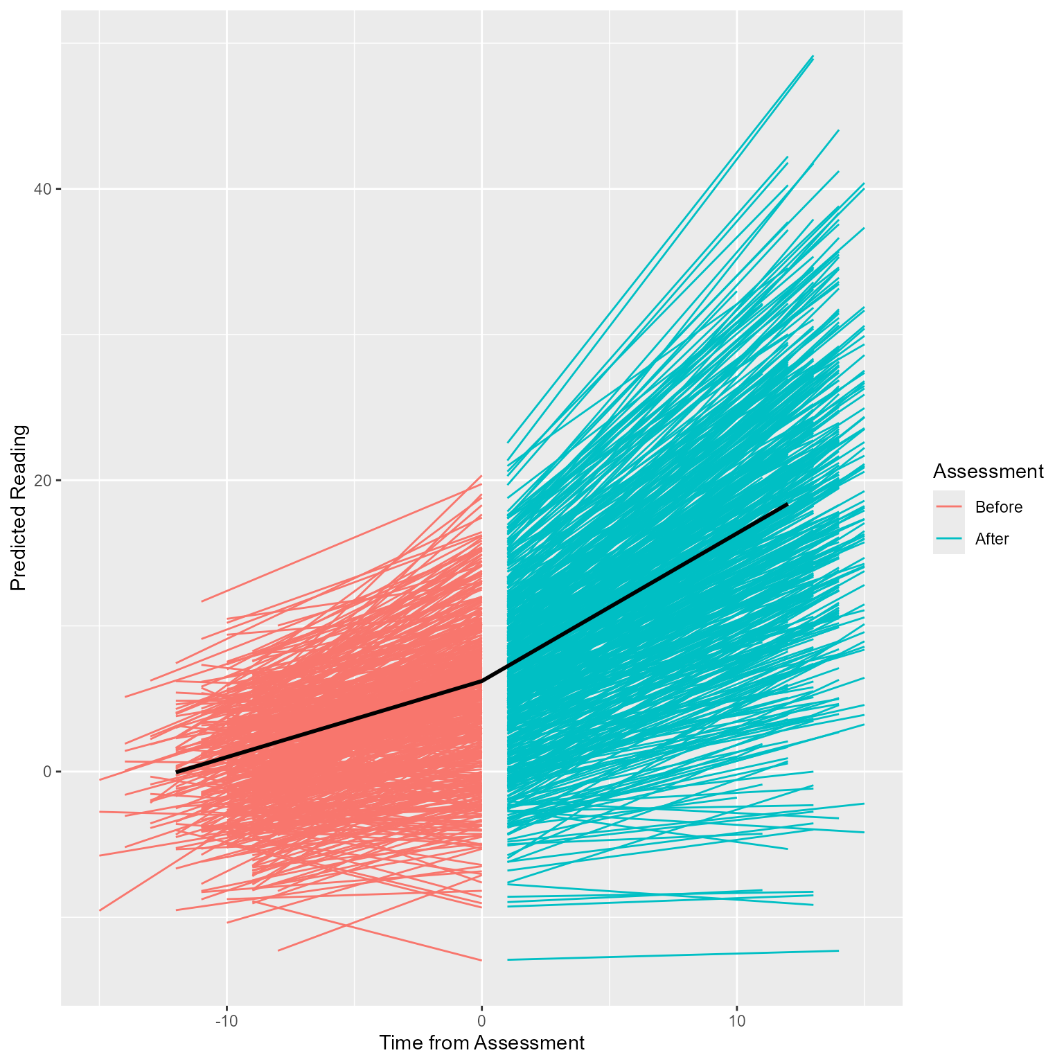
Yes! The rate of improvement becomes steeper after the assessment. Now that we know that the data generation has the effect we want, we can detect the effect analytically.

Effect Detection Function

Here we run the analysis, extract the t statistic for months_after_assessment, and return TRUE or FALSE depending if t > 2. We could extract an exact p-value and test whether it is less than 0.05, but that is not necessary here.

fit_model <- function(data) {
  lme4::lmer(reading ~ month + months_after_assessment + (1 + month | student_id), data = data)
}

detect_effect <- function(fit) {
  broom.mixed::tidy(fit, effects = "fixed", conf.int = TRUE) %>%
    mutate(significant = 1 * (conf.low * conf.high > 0)) %>% 
    select(term, significant)
}

Generate Many Data Sets, Detecting the Effect on Each Set

Our detect_effect function returns TRUE or FALSE.

The replicate function will perform detect_effect with our specified settings as many times as we want. It normally returns a vector if it can, but with simplify = FALSE it will return a list of all the objects created by our analysis. This list is bound into a single data.frame with bind_rows and then filtered to remove the intercept. Finally, we summarize the results by taking the mean of the significant column.

# Fixed effects
b_00 = 0 # Reading level at month 0
b_10 = 0.5 # Pre-assessment growth rate
b_20 = 0.25 # Assessment effect on growth rate


# Level-2 random effects covariance matrix
tau <- lavaan::lav_matrix_lower2full(c(tau_00 = 16,
                                       tau_10 = 0, tau_11 = 0.16))

# Number of times to replicate
k_replications <- 100

# Estimate power 
replicate(k_replications, make_data(n = 100, 
                             b_00 = b_00,
                             b_10 = b_10,
                             b_20 = b_20,
                             sigma_e = 2, 
                             tau_00 = tau_00, 
                             tau_11 = tau_11,
                             r_01 = r_01,
                             k_months_total = 12,
                             k_months_before = 4,
                             k_months_delay = 2) %>% 
            fit_model() %>% 
            detect_effect(),
          simplify = FALSE) %>% 
  bind_rows() %>% 
  filter(term != "(Intercept)") %>% 
  summarise(significant = mean(significant), .by = term)

# A tibble: 2 × 2
  term                    significant
  <chr>                         <dbl>
1 month                          1   
2 months_after_assessment        0.93

I usually start with a small number of replications (e.g., 10) to make sure the function is working as intended. Then I increase the replications by powers of 10 (100, 1000, 10000) until the analysis produces stable estimates and does not take too long to run.

We can play around with different samples sizes we are interested in (50, 100, 200, 300, 500, 1000, …).

An Alternate “Tidy” Method

Here we create a tibble with 1000 rows, each with a different sample size between 20 and 200. We create a new variable called Power that will contain the output of a function that makes data and tells us whether the effect was detected. The map_dbl is part of the map family. It takes the input of our sample size column n and performs our custom function for every row. The Power variable is just a column of 1s and 0s, telling whether the effect was detected or not.

I then plot the results using the geom_smooth function. I specify a binomial glm, which is a logistic regression—regression for binary output. The result is a plot showing the relationship between sample size and power.

tibble(n = 20:200) %>%
  mutate(Power = map(n, \(n) {
    make_data(
      n = n,
      b_00 = b_00,
      b_10 = b_10,
      b_20 = b_20,
      sigma_e = 2,
      tau_00 = tau_00,
      tau_11 = tau_11,
      r_01 = r_01,
      k_months_total = 12,
      k_months_before = 4,
      k_months_delay = 2
    ) %>%
      fit_model() %>%
      detect_effect()
  })) %>%
  unnest(Power) %>% 
  filter(term != "(Intercept)") %>% 
  ggplot(aes(n, significant)) +
  geom_smooth(method = "glm",
              method.args = list(family = "binomial"), se = FALSE) + 
  geom_hline(yintercept = .9) +
  facet_wrap(vars(term)) + 
  scale_y_continuous(limits = c(0,1), breaks = seq(0,1,.2))

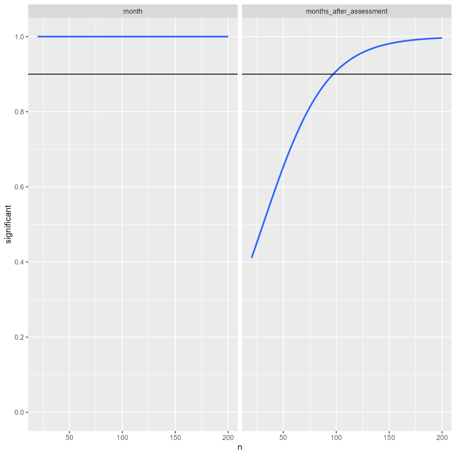
Given the assumptions I set up, 90% power for the month variable is present in even small sample sizes. For the months_after_assessment variable, 90% power is present at a sample size of about 75.

Suppose that I am not so sure about the size of assessment’s effect. Therefore, I specify a variety of effect sizes for b_{20}. The crossing function creates tibble with all combinations of n and b_20. I then set repeats to 2, so that I can see the effect of sample size and effect size on power. The uncount function creates a new row for each row in the tibble, repeating the rows by the number of times specified in repeats.

crossing(n = c(seq(10,90, 5), seq(100, 1000, 25)), 
         b_20 = c(Smaller = .1,
                      Medium = .2,
                      Larger = .3)) %>% 
  mutate(repeats = 2,
         `Effect Size` = paste0(names(b_20),
                                " (",
                                b_20, 
                                ")")) %>%
  uncount(repeats) %>% 
  mutate(Power = map2(n, b_20, \(nn, bb_20) {
   make_data(
      n = nn,
      b_00 = b_00,
      b_10 = b_10,
      b_20 = bb_20,
      sigma_e = 2,
      tau_00 = tau_00,
      tau_11 = tau_11,
      r_01 = r_01,
      k_months_total = 12,
      k_months_before = 4,
      k_months_delay = 2
    ) %>%
      fit_model() %>%
      detect_effect()
  })) %>%
  unnest(Power) %>% 
  filter(term != "(Intercept)") %>% 
  ggplot(aes(n, significant)) + 
  geom_smooth(method = "glm", se = F,
              method.args = list(family = "binomial"), 
              aes(color = `Effect Size`)) +
  scale_x_log10("Sample Size (log)", breaks = c(1, 10,seq(20,100, 20), seq(200, 1000, 200))) + 
    geom_hline(yintercept = .9) +
  theme(legend.position = c(1,0), legend.justification = c(1,0)) +
  scale_color_viridis_d(end = .9, begin = .1) + 
  scale_y_continuous(breaks = seq(0,1,0.2)) +
   facet_wrap(vars(term))

Figure 1: Power Analysis by Sample Size and Effect Size

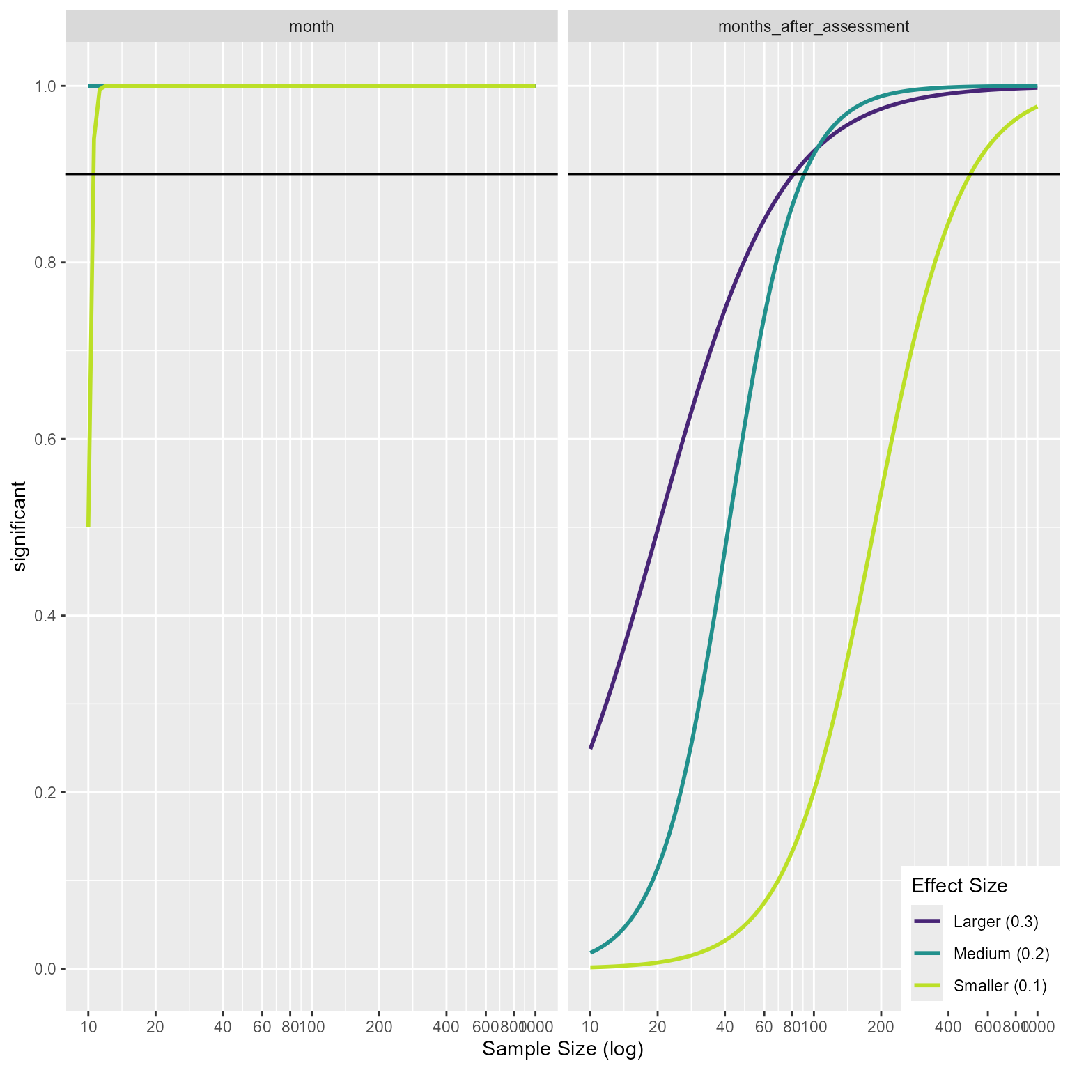
Thus, it appears that under the assumptions my model has, I can detect my effect with around 100 or fewer when the effect of assessment is greater than 0.2. If the effect is 0.1, I would need about 500 participants to detect the effect with reasonable power.

In the same way that we varied the sample size and effect size, we can vary any other parameter we want (e.g., number of measurements, length of time before the assessment) and plot the how these factors influence power.