The psycheval package is a set of functions that can be useful in psychological evaluations. It accompanies the Individual Psychometrics online textbook.
Convert a variable to standard scores
Suppose you have a scaled score of 12 (μ = 10, σ = 3) that you want to convert to a standard score (μ = 100, σ = 15).
library(psycheval)
x2standard(12, mu_x = 10, sigma_x = 3)
#> [1] 110
To convert to a z-score (μ = 0, σ = 1):
x2standard(12,
           mu_x = 10, sigma_x = 3,
           mu_new = 0, sigma_new = 1)
#> [1] 0.67
To convert to T-score (μ = 50, σ = 10):
x2standard(12,
           mu_x = 10, sigma_x = 3,
           mu_new = 50, sigma_new = 10)
#> [1] 57
Covariance of weighted sums
Let’s create a covariance matrix of 5 variables that all correlate at .60.
# Create covariance matrix
Sigma <- matrix(0.6, nrow = 5, ncol = 5)
diag(Sigma) <- 1
Sigma
#>      [,1] [,2] [,3] [,4] [,5]
#> [1,]  1.0  0.6  0.6  0.6  0.6
#> [2,]  0.6  1.0  0.6  0.6  0.6
#> [3,]  0.6  0.6  1.0  0.6  0.6
#> [4,]  0.6  0.6  0.6  1.0  0.6
#> [5,]  0.6  0.6  0.6  0.6  1.0
Suppose we want to create a sum of the first 2 variables and a sum of the remaining three variables. What would the covariance matrix of the summary variables be?
First we create a weight matrix w with 5 rows and 2 columns consisting entirely of zeros. The first column represents the weight for the first variable. We put ones in the first two rows of the first column and ones in rows 3–5 in the second column.
# Create weight matrix
w <- matrix(0, nrow = 5, ncol = 2)
w[1:2,1] <- 1
w[3:5,2] <- 1
w
#>      [,1] [,2]
#> [1,]    1    0
#> [2,]    1    0
#> [3,]    0    1
#> [4,]    0    1
#> [5,]    0    1
Composite covariance
The covariance matrix of the sums is:
# covariance matrix of weighted sums
composite_covariance(Sigma, w)
#>      [,1] [,2]
#> [1,]  3.2  3.6
#> [2,]  3.6  6.6
To include the original variables in the covariance matrix, append an identity matrix to w:
# A 5 by 5 idendity matrix
I <- diag(5)
I
#>      [,1] [,2] [,3] [,4] [,5]
#> [1,]    1    0    0    0    0
#> [2,]    0    1    0    0    0
#> [3,]    0    0    1    0    0
#> [4,]    0    0    0    1    0
#> [5,]    0    0    0    0    1

# Prepend the identity matrix to the w matrix
w_expanded <- cbind(diag(5), w)
w_expanded
#>      [,1] [,2] [,3] [,4] [,5] [,6] [,7]
#> [1,]    1    0    0    0    0    1    0
#> [2,]    0    1    0    0    0    1    0
#> [3,]    0    0    1    0    0    0    1
#> [4,]    0    0    0    1    0    0    1
#> [5,]    0    0    0    0    1    0    1

# Covariance matrix of original variables and the summary variables
BigSigma <- composite_covariance(Sigma, w_expanded)
BigSigma
#>      [,1] [,2] [,3] [,4] [,5] [,6] [,7]
#> [1,]  1.0  0.6  0.6  0.6  0.6  1.6  1.8
#> [2,]  0.6  1.0  0.6  0.6  0.6  1.6  1.8
#> [3,]  0.6  0.6  1.0  0.6  0.6  1.2  2.2
#> [4,]  0.6  0.6  0.6  1.0  0.6  1.2  2.2
#> [5,]  0.6  0.6  0.6  0.6  1.0  1.2  2.2
#> [6,]  1.6  1.6  1.2  1.2  1.2  3.2  3.6
#> [7,]  1.8  1.8  2.2  2.2  2.2  3.6  6.6

# Convert to correlations with the cov2cor function
composite_covariance(Sigma, w_expanded, correlation = T)
#>        [,1]   [,2]   [,3]   [,4]   [,5]   [,6]   [,7]
#> [1,] 1.0000 0.6000 0.6000 0.6000 0.6000 0.8944 0.7006
#> [2,] 0.6000 1.0000 0.6000 0.6000 0.6000 0.8944 0.7006
#> [3,] 0.6000 0.6000 1.0000 0.6000 0.6000 0.6708 0.8563
#> [4,] 0.6000 0.6000 0.6000 1.0000 0.6000 0.6708 0.8563
#> [5,] 0.6000 0.6000 0.6000 0.6000 1.0000 0.6708 0.8563
#> [6,] 0.8944 0.8944 0.6708 0.6708 0.6708 1.0000 0.7833
#> [7,] 0.7006 0.7006 0.8563 0.8563 0.8563 0.7833 1.0000
Compute a composite score
Suppose we have two subtest scores A = 12 and B = 14. Both scores are on the scaled score metric (μ = 10, σ = 3). We want to create a composite score on the standard score metric (μ = 100, σ = 15).
The subtests A and B correlated at ρ = .6.
# Subtest scores
x <- c(12, 14)

# Subtest correlation
rho <- 0.6

# Subtest correlation matrix
R <- matrix(c(1,rho, rho, 1), ncol = 2)

# Compute composite score
composite_score(x = x,
                R = R,
                mu_x = 10,
                sigma_x = 3,
                mu_composite = 100,
                sigma_composite = 15)
#> [1] 116.8
Compute a multivariate confidence interval conditioned on a set of observed scores
library(readr)
library(ggplot2)
library(dplyr)
#>
#> Attaching package: 'dplyr'
#> The following objects are masked from 'package:stats':
#>
#>     filter, lag
#> The following objects are masked from 'package:base':
#>
#>     intersect, setdiff, setequal, union

# Observed scores
x_wisc <- c(
  vci = 130,
  vsi = 120,
  fri = 123,
  wmi = 116,
  psi = 97)

# Reliability coefficients
rxx_wisc <- c(
  vci = .92,
  vsi = .92,
  fri = .93,
  wmi = .92,
  psi = .88)

# Correlation matrix
R_wisc <- ("
  index vci     vsi     fri     wmi     psi
  vci   1.00    0.59    0.59    0.53    0.30
  vsi   0.59    1.00    0.62    0.50    0.36
  fri   0.59    0.62    1.00    0.53    0.31
  wmi   0.53    0.50    0.53    1.00    0.36
  psi   0.30    0.36    0.31    0.36    1.00") |>
  read_tsv(col_types = cols(
    .default = col_double(),
    index = col_character())) |>
  tibble::column_to_rownames("index") |>
  as.matrix()
R_wisc
#>      vci  vsi  fri  wmi  psi
#> vci 1.00 0.59 0.59 0.53 0.30
#> vsi 0.59 1.00 0.62 0.50 0.36
#> fri 0.59 0.62 1.00 0.53 0.31
#> wmi 0.53 0.50 0.53 1.00 0.36
#> psi 0.30 0.36 0.31 0.36 1.00

d_ci <- multivariate_ci(
  x = x_wisc,
  r_xx = rxx_wisc,
  mu = rep(100, 5),
  sigma = R_wisc * 225)

d_ci
#>     variable   x r_xx mu_univariate see_univariate mu_multivariate
#> vci      vci 130 0.92        127.60          4.069          127.88
#> vsi      vsi 120 0.92        118.40          4.069          119.70
#> fri      fri 123 0.93        121.39          3.827          122.33
#> wmi      wmi 116 0.92        114.72          4.069          115.95
#> psi      psi  97 0.88         97.36          4.874           98.86
#>     see_multivariate upper_univariate lower_univariate upper_multivariate
#> vci            3.912            135.6           119.62              135.5
#> vsi            3.897            126.4           110.42              127.3
#> fri            3.685            128.9           113.89              129.6
#> wmi            3.954            122.7           106.74              123.7
#> psi            4.803            106.9            87.81              108.3
#>     lower_multivariate
#> vci             120.21
#> vsi             112.07
#> fri             115.11
#> wmi             108.20
#> psi              89.44
Compare the multivariate CI to the univariarte CI:
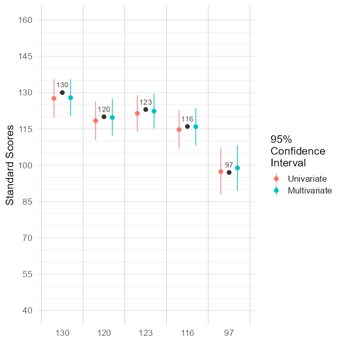
Multivariate Confidence Intervals
Relative Proficiency Index
When a typical same-age peer with an ability of W = 500 has a .90 probability of answering a question correctly, what is the probability that a person with ability of W = 520 will answer the question correctly?
rpi(x = 520, mu = 500)
#> 0.9878
Flipping the previous question, when a person with ability of W = 520 has a .90 probability of answering a question correctly, what is the probability that a typical same-age peer with an ability of W = 500 will answer the question correctly?
rpi(x = 520, mu = 500, reverse = TRUE)
#> 0.5
Criteria other than .9 proficiency are also possible. For example, when a typical same-age peer with an ability of W = 500 has a .25 probability of answering a question correctly, what is the probability that a person with ability of W = 520 will answer the question correctly?
rpi(x = 520, mu = 500, criterion = .25)
#> 0.75