Latent Variable Models
Latent growth modeling is a specific instance of a more general approach to creating models with a mix of observed and latent variables. This approach goes by many names, including latent variable modeling , structural equation modeling , covariance structure analysis , and many other similar terms.
Latent variables are not observed directly but are inferred from the patterns of relationships among observed variables. For example, suppose we see that three different vocabulary tests, v1 , v2 , v3 , have the correlations in Table 1 .
Code
<- "V =~ .7 * v_1 + .8 * v_2 + .9 * v_3" :: get_model_implied_correlations (m) %>% :: as_cordf (diagonal = 1 ) %>% mutate (term = paste0 (str_replace (paste0 ("*" , toupper (term), "*" ), "_" , "~" ), "~" )) %>% rename (` ` = term) %>% mutate (across (where (is.numeric), round_probability)) %>% :: gt () %>% my_apa () %>% :: fmt_markdown () %>% :: cols_label (v_1 = md ("*V*~1~" ),v_2 = md ("*V*~2~" ),v_3 = md ("*V*~3~" )%>% :: cols_width (` ` ~ px (50 ),everything () ~ px (70 )) %>% :: cols_align (columns = 2 : 4 , "center" )
V1 1
.56
.63
V2 .56
1
.72
V3 .63
.72
1
Table 1: Correlations Among Three Vocabulary Tests
What underlying model would create these correlations? Unfortunately, any set of observed correlations could be generated from an infinite number of models. Of the infinite number of models that could generate these correlations, most of them have no theoretical basis and are stuffed with unnecessary complications. When deciding among alternatives, a good place to start is to imagine the simplest theoretically plausible explanation. As Einstein is reputed to have said ,
“Everything should be made as simple as possible, but not simpler.”
Code
ggdiagram (font_size = 24 , font_family = my_font) + <- ob_circle (label = "*Vocabulary*" , radius = sqrt (pi))} + <- ob_ellipse (m1 = 15 ) %>% place (v, "below" , sep = 2 ) %>% ob_array (k = 3 ,sep = .25 ,label = paste0 ("*V*~" , 1 : 3 , "~" ))} + <- connect (v, v3, resect = 2 )} + ob_label (label = round_probability (seq (.7 , .9 , .1 ), phantom_text = "." ),center = l@ line@ point_at_y (l[2 ]@ midpoint (.47 )@ y),size = 20 ,label.padding = margin (t = 4 , b = 0 )) + <- ob_circle (label = paste0 ("*e*~" , 1 : 3 , "~" ), radius = .75 ) %>% place (v3, "below" , sep = .75 )} + connect (e3, v3, resect = 2 ) + ob_variance (x = e3,where = "below" ,looseness = 1.25 ,label = ob_label (label = round_probability (1 - seq (.7 , .9 , .1 )^ 2 ), size = 18 )) + ob_variance (label = ob_label ("1" , size = 18 ),theta = 40 ,looseness = .8 )
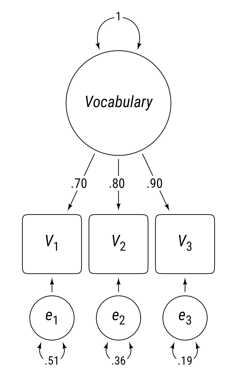
In this case, the simplest theoretically plausible model I can imagine is that people have an overall fund of knowledge about words in a particular language and that each vocabulary test score samples this knowledge imperfectly. In Figure 1 , the circle labeled Vocabulary is a latent variable that represents the influence of an overall knowledge of words. It is latent because there is no practical way to measure a person’s overall knowledge of words. At best, we create tests that sample this overall knowledge with a subset of words we believe are representative of the overall word knowledge. Observed variables are represented in Figure 1 as squares. People with a large overall vocabulary are likely to score well on the three measures of vocabulary we have created. People with a small vocabulary will likely score lower on the three tests.
Sidenote : Is the true model that generated the correlation matrix in Table 1 more complex than the simple model in Figure 1 ? Undoubtedly. We generate simple models as a starting point in our investigation, as a basis of comparison for subsequent models.The influence of the latent variable on the observed indicator variable is symbolized by a straight arrow. The strength of the influence is called a loading . Observed variables with stronger loadings are better indicators of the latent variable. Because the loadings are standardized (i.e., all observed and latent variables have a variance of 1), the loadings in this context equal the correlation between the latent variable and each observed variable.
1 Standardized loadings are actually standardized regression coefficients from latent variables to observed variables. When an observed variable has only one loading and no other influences (other than the error term), the standardized regression coefficient equals the correlation between the latent variable and the observed indicator.
Although the three tests are influenced by a common cause, in Figure 1 , each tests has a unique set of influences, e 1 , e 2 , e 3 . The variances of the unique influences are symbolized by curved double-headed arrows. Because they are standardized, they represent the proportion of variance in the observed variables that is not explained by the latent variable.
The model in Figure 1 has 1 latent variable, 3 observed variables, and 3 error/residual terms. Any variable that has an incoming straight arrow from another variable is said to be endogenous , meaning “created from within” the model. That is, endogenous variables are determined entirely be variables within the model. A variable without incoming straight arrows is said to be exogenous , meaning “created from without.” That is, exogenous variables are random variables that are determined by influences not specified by the model. In Figure 1 , the three observed variables V_1, V_2, V_3 each have two incoming straight arrows, thus they are endogenous. The latent variable \text{Vocabulary} and the three error terms e_1, e_2, e_3 have no incoming straight arrows from other variables, thus they are exogenous.
2 In some latent variable models, means of exogneous variables and intercepts of endogenous variables are symbolized by paths originating from a triangle. Thus, exogenous variables can have incoming arrows from triangles and still be considered exogenous because such arrows simply specify the mean of the variable and do not determine their variability.
McArdle, J. J., & McDonald, R. P. (1984). Some algebraic properties of the
Reticular Action Model for moment structures.
British Journal of Mathematical and Statistical Psychology ,
37 (2), 234–251.
https://doi.org/10.1111/j.2044-8317.1984.tb00802.x
We can specify latent variable models in a variety of ways, but simplest method, the Reticular Action Model (McArdle & McDonald, 1984 ) , uses two matrices \boldsymbol{A} (Asymmetric) and \boldsymbol{S} (Symmetric). The \boldsymbol{A} matrix contains the asymmetric paths (i.e., single-headed straight arrows). These paths quantify how much latent and observed variables influence each other. In the current model, the only straight arrows are from the latent variable to the observed variables.
Code
tibble (Effects = c ("*Vocabulary*" , "*V*~1~" , "*V*~2~" , "*V*~3~" ),V = c ("0" , ".7" , ".8" , ".9" ),v1 = c (0 , 0 , 0 , 0 ),v2 = c (0 , 0 , 0 , 0 ),v3 = c (0 , 0 , 0 , 0 )%>% :: gt () %>% my_apa () %>% :: fmt_markdown () %>% :: cols_label (v1 = md ("*V*~1~" ),v2 = md ("*V*~2~" ),v3 = md ("*V*~3~" ),V = md ("*Vocabulary*" ),Effects = md ("**Effects**" )%>% :: cols_align (align = "right" , columns = 1 ) %>% :: cols_align (align = "center" , columns = 2 : 5 ) %>% :: tab_spanner (columns = starts_with ("v" ), label = md ("**Causes**" ))
Vocabulary V 1 V 2 V 3
Vocabulary 0
0
0
0
V 1 .7
0
0
0
V 2 .8
0
0
0
V 3 .9
0
0
0
Table 2: \boldsymbol{A} Matrix::Asymmetric Paths from Causes to Effect in Figure 1
The \boldsymbol{S} matrix contains the symmetric paths (i.e., double-headed curved arrows). These quantify the variances of the exogenous variables and the covariances between them. In this case, all the covariances among the exogenous variables are zero. The variances were standardized such that the latent variable has a variance of 1 and the variances of the error terms were selected to cause the variances of the observed variances to be exactly 1.
Code
tibble (` ` = c ("*Vocabulary*" , "*e*~1~" , "*e*~2~" , "*e*~3~" ),` Vocabulary ` = c (1 , 0 , 0 , 0 ),e1 = c (0 , ".51" , 0 , 0 ),e2 = c (0 , 0 , ".36" , 0 ),e3 = c (0 , 0 , 0 , ".19" )) %>% :: gt () %>% my_apa () %>% :: fmt_markdown () %>% :: cols_label (e1 = md ("*e*~1~" ),e2 = md ("*e*~2~" ),e3 = md ("*e*~3~" ),Vocabulary = md ("*Vocabulary*" )) %>% :: cols_align (align = "right" , columns = 1 ) %>% :: cols_align (align = "center" , columns = 2 : 5 ) %>% :: cols_width (everything () ~ px (100 )) %>% :: tab_spanner (columns = starts_with ("e" ), label = md ("**Errors**" )) %>% :: tab_spanner (columns = "Vocabulary" , label = md ("**Latent**" ))
Vocabulary e 1 e 2 e 3
Vocabulary 1
0
0
0
e 1 0
.51
0
0
e 2 0
0
.36
0
e 3 0
0
0
.19
Table 3: \boldsymbol{S} Matrix: Symmetric Paths Among Exogenous Varibles in Figure 1
The two matrices, \boldsymbol{A} and \boldsymbol{S} jointly determine the model-implied covariance matrix \boldsymbol{\Sigma} . If the latent and observed variables are collected in a vector v=\{Vocabulary, v_1, v_2, v_3\} , and the exogenous variables are collected in a vector u=\{Vocabulary, e_1, e_2, e_3\} , then we can specify how the variables in v influence each other like so:
\begin{aligned}
v&=\boldsymbol{A}v+u\\[3ex]
\begin{bmatrix}
Vocabulary\\ V_1\\ V_2\\ V_3
\end{bmatrix}&=
\begin{bmatrix}
0&0&0&0\\
.7&0&0&0\\
.8&0&0&0\\
.9&0&0&0
\end{bmatrix}\begin{bmatrix}
Vocabulary\\ V_1\\ V_2\\ V_3
\end{bmatrix}+\begin{bmatrix}
Vocabulary\\ e_1\\ e_2\\ e_3
\end{bmatrix}
\end{aligned}
It might feel strange to have the v variable on both sides of the equation. Remember that it is not a single variable, but a vector of variables. The \boldsymbol{A} matrix specifies how the causes in v influence the effects in v . Even so, it helps to isolate v on one side of the equation. We will make use of an identity matrix I in which the diagonal values are ones and the off-diagonal values are zeroes.
I=\begin{bmatrix}
1&0&0&0\\
0&1&0&0\\
0&0&1&0\\
0&0&0&1
\end{bmatrix}
An identity matrix is so-named because any matrix multiplied by a compatible identity matrix equals itself.
\boldsymbol{A}\boldsymbol{I}=\boldsymbol{A}
To be compatible when post-multiplied, \boldsymbol{I} would need to have the same size as the number of columns in A.
\boldsymbol{I}\boldsymbol{A}=\boldsymbol{A}
To be compatible when pre-multiplied, \boldsymbol{I} would need to have the same size as the number of rows in A.
We will also use an inverse matrix. A matrix multiplied by its inverse matrix will equal a same-sized identity matrix.
\boldsymbol{A}\boldsymbol{A}^{-1}=\boldsymbol{I}
So, starting with the original equation:
\begin{aligned}
v&=\boldsymbol{A}v +u\\
v-\boldsymbol{A}v&=u\\
\boldsymbol{I}v-\boldsymbol{A}v&=u\\
(\boldsymbol{I}-\boldsymbol{A})v&=u\\
(\boldsymbol{I}-\boldsymbol{A})^{-1}(\boldsymbol{I}-\boldsymbol{A})v&=(\boldsymbol{I}-\boldsymbol{A})^{-1}u\\
\boldsymbol{I}v&=(\boldsymbol{I}-\boldsymbol{A})^{-1}u\\
v&=(\boldsymbol{I}-\boldsymbol{A})^{-1}u\\[3ex]
\begin{bmatrix}
Vocabulary\\ V_1\\ V_2\\ V_3
\end{bmatrix}&=
\begin{bmatrix}
1&0&0&0\\
.7&1&0&0\\
.8&0&1&0\\
.9&0&0&1
\end{bmatrix}\begin{bmatrix}
Vocabulary\\ e_1\\ e_2\\ e_3
\end{bmatrix}
\end{aligned}
So, the variables in v are determined by exogenous variables in u pre-multiplied by the inverse of (\boldsymbol{I}-\boldsymbol{A}) . This matrix equation equals this in univariate equations:
\begin{aligned}
Vocabulary &= Vocabulary\\
V_1 &= .7Vocabulary+e_1\\
V_2 &= .8Vocabulary+e_2\\
V_2 &= .9Vocabulary+e_2\\
\end{aligned}
The \boldsymbol{S} matrix is the model-implied variance-covariance matrix of u :
\begin{aligned}\
\boldsymbol{S}&=\mathcal{E}\left(uu'\right)\\
&=\mathrm{Cov}(u)
\end{aligned}
The \boldsymbol{\Sigma} matrix is the model-implied variance-covariance matrix of v :
\begin{aligned}\
\boldsymbol{\Sigma} &=\mathcal{E}\left(vv'\right)\\
&= \mathrm{Cov}\left(v\right)\\
&=\mathrm{Cov}\left(\left(\boldsymbol{I}-\boldsymbol{A}\right)^{-1}u\right)\\
&=\left(\boldsymbol{I}-\boldsymbol{A}\right)^{-1}\boldsymbol{S}\left(\left(\boldsymbol{I}-\boldsymbol{A}\right)^{-1}\right)'
\end{aligned}
If we have the values of matrices \boldsymbol{A} and \boldsymbol{S} , then the model-implied covariance matrix \boldsymbol{\Sigma} can be calculated directly:
# factor loadings <- c (.7 , .8 , .9 )# Asymmetric <- matrix (0 , nrow = 4 , ncol = 4 )2 : 4 ,1 ] <- loadings# Symmetric, diag makes a diagonal matrix <- diag (c (1 , 1 - loadings ^ 2 ))# Identity, diag(4) makes a 4 by 4 identity matrix <- diag (4 )# Inverse matrix, solve inverts matrices <- solve (I - A)# Model-implied correlations, %*% is matrix multiplication <- iA %*% S %*% t (iA)
Code
%>% ` colnames<- ` (c ("Vocabulary" , "v1" , "v2" , "v3" )) %>% ` rownames<- ` (c ("Vocabulary" , "*V*~1~" , "*V*~2~" , "*V*~3~" )) %>% as.data.frame () %>% :: rownames_to_column (" " ) |> mutate (across (where (is.numeric), ggdiagram:: round_probability)) %>% :: gt () %>% my_apa () %>% :: fmt_markdown () %>% :: cols_label (v1 = md ("*V*~1~" ),v2 = md ("*V*~2~" ),v3 = md ("*V*~3~" )) %>% :: cols_align (align = "center" ) %>% :: cols_align ("right" , 1 ) %>% :: cols_width (everything () ~ gt:: px (100 )) %>% :: tab_spanner (columns = paste0 ("v" , 1 : 3 ), label = md ("**Observed**" )) %>% :: tab_spanner (columns = "Vocabulary" , label = md ("**Latent**" ))
Vocabulary
V 1 V 2 V 3
Vocabulary
1
.70
.80
.90
V 1 .70
1
.56
.63
V 2 .80
.56
1
.72
V 3 .90
.63
.72
1
Table 4: The model-implied correlation matrix
Most of the time, we do not know the values of \boldsymbol{A} and \boldsymbol{S} . We have instead the means, standard deviations, and correlations of the observed variables. Using specialized syntax to specify a model, the lavaan package can estimate the values of \boldsymbol{A} and \boldsymbol{S} of that model that have a model-implied covariance matrix is as close to the observed covariance matrix as possible.
If the estimated values of \boldsymbol{A} and \boldsymbol{S} can closely duplicate the observed covariances, then the model is not necessarily correct, but is more plausible than a model that cannot closely duplicate the observed covariances. Researchers try to find the simplest theory-based model that “fits” the data. In this context, the model “fits” the data when the model-implied covariance matrix closely resembles the observed covariances.
lavaan Syntax Overview
We will be using the lavaan (LA tent VA riable AN alysis) package to conduct latent growth modeling analyses. To have lavaan evaluate a model, you need to tell it which model you want to test. The lavaan package has a special syntax for specifying models (basic syntax , advanced syntax ). The aspects of lavaan syntax relevant to this tutorial are in Table 5 .
=~A =~ A1 + A2Latent variable A has observed indicators A1 and A2.
~Y ~ X1 + X2Y is predicted by X1 and X2.
Y ~ a * X1 + a * X2Make X1 and X2 coefficients equal.
Y ~ 1 * X1 + X2Set the regression coefficient of X1 to 1.
~~X1 ~~ X2Estimate the covariance between X1 and X2.
X1 ~~ 0.5 * X2Set the covariance between X1 and X2 to 0.5.
X1 ~~ 1 * X1Set X1’s variance to 1.
Table 5: Syntax for lavaan models
In lavaan, latent variable indicators are specified with the =~ operator, which means is indicated by . Consider this lavaan model:
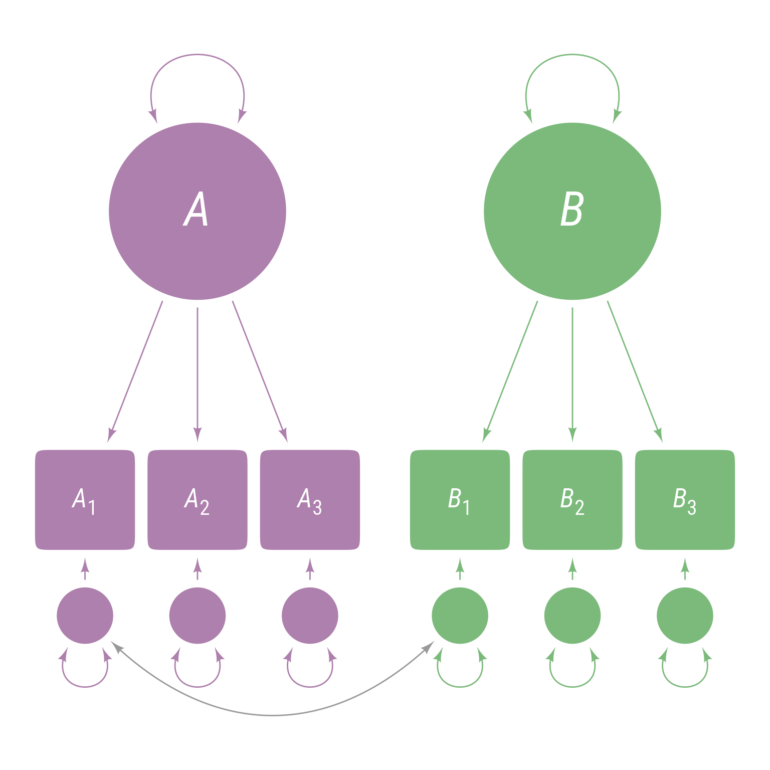
<- ' A =~ A1 + A2 + A3 B =~ B1 + B2 + B3 '
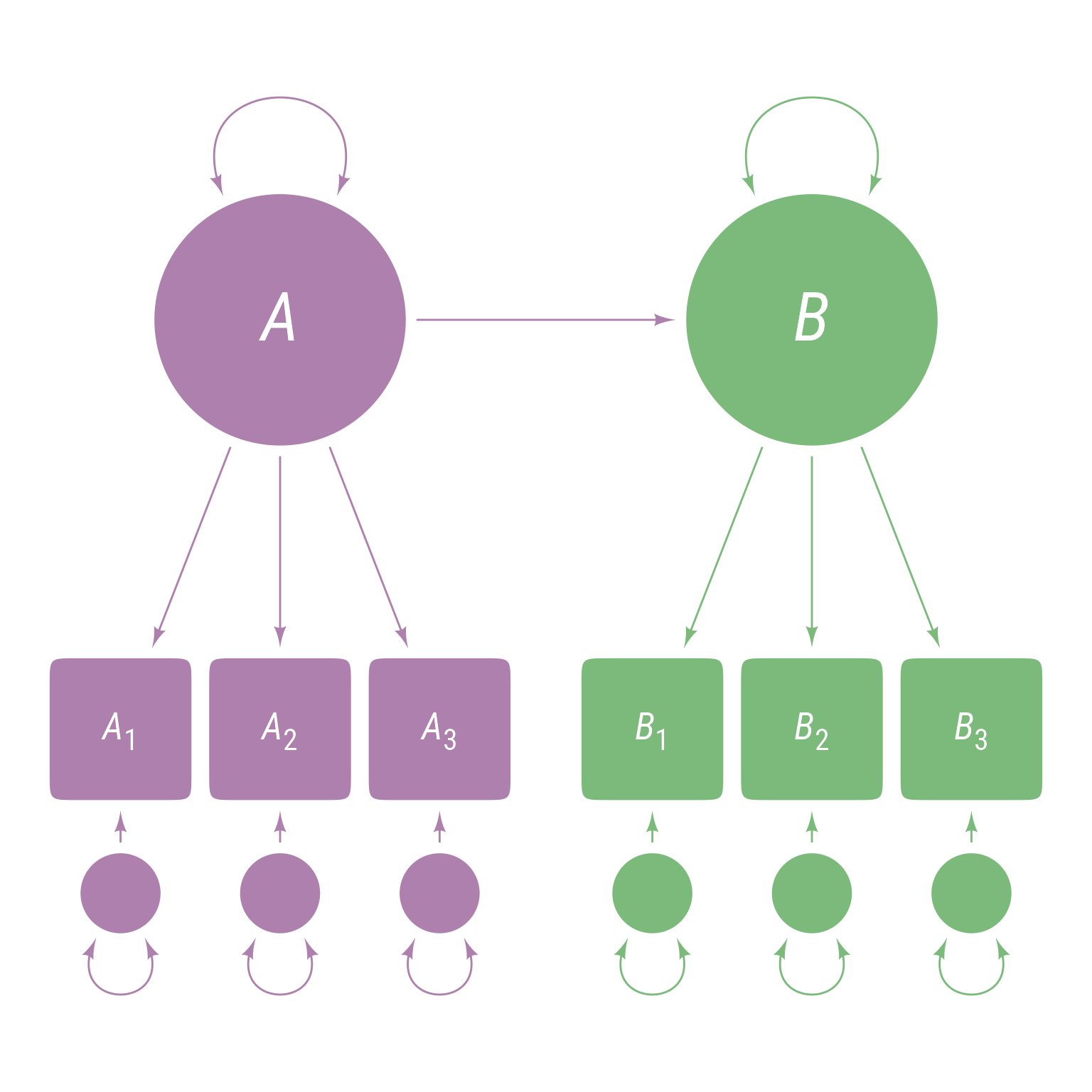
This model means there are 3 observed variables A1, A2, and A3 that are indicators of latent variable A and 3 observed variables B1, B2, and B3 that are indicators of latent variable B. The model hypothesizes that latent variable A explains the correlations among A1, A2, and A3 and that latent variable B explains the correlations among B1, B2, and B3. The corresponding path model is in Figure 2 . Note that the latent variables A and B are uncorrelated because there is nothing to connect them, which means that A1, A2, and A3 are uncorrelated with B1, B2, and B3.
Code
<- class_color ("orchid4" )@ lighten (.7 )<- class_color ("forestgreen" )@ lighten (.6 )<- class_color ("dodgerblue4" )@ lighten (.6 )<- "#b5bdc7" <- 7 <- c (cA, cB, cC)<- redefault (ob_ellipse, m1 = 15 , color = NA , fill = cA)<- redefault (ob_circle, radius = sqrt (pi), color = NA , fill = cA)<- redefault (ob_circle, radius = 1 / sqrt (pi), color = NA , fill = cA)<- redefault (connect, color = cA, resect = 2 )<- redefault (ob_label, color = "white" ,fill = NA , size = 20 , vjust = .60 )<- redefault (ob_label, color = "white" ,fill = NA , size = 36 , vjust = .55 )<- redefault (ob_label,fill = NA ,color = "white" ,size = 16 )<- ggdiagram (font_family = my_font, font_size = 20 ) + <- my_observed () %>% ob_array (k = 3 ,label = my_observed_label (paste0 ("*A*~" , 1 : 3 , "~" )),sep = .25 )} + <- my_observed (fill = cB) %>% place (A3[3 ], sep = 0 ) %>% ob_array (3 ,anchor = "west" ,label = my_observed_label (paste0 ("*B*~" , 1 : 3 , "~" )sep = .25 )} + <- my_latent (label = my_latent_label ("*A*" )) %>% place (A3[2 ], "above" , 3 )} + <- my_latent (fill = cB,label = my_latent_label ("*B*" )%>% place (B3[2 ], "above" , 3 )} + <- my_connect (A, A3)} + <- my_connect (B, B3, color = cB)} + <- ob_variance (A, color = cA)} + <- ob_variance (B, color = cB)} + <- my_error () %>% ob_array (3 ) %>% place (A3, "below" , sep = .75 ) } + <- my_error (fill = cB) %>% place (B3, "below" , sep = .75 )} + ob_variance (eA3, color = cA, where = "below" , theta = 60 , looseness = 2 ) + ob_variance (eB3, color = cB, where = "below" , theta = 60 , looseness = 2 ) + my_connect (eA3, A3) + my_connect (eB3, B3, color = cB)
Figure 2: Path diagram of latent variables A and B, each of which have three observed indicator variables
To specify that an indicator has a specific (fixed) loading, do so by placing the numeric loading in front of the variable with the * operator in between. Here we set the loadings for A1 and B1 to 1:
<- ' A =~ 1 * A1 + A2 + A3 B =~ 1 * B1 + B2 + B3 '
The corresponding path model is in Figure 3 .
Code
+ ob_label ("1" , center = midpoint (A, A3[1 ]), color = cA) + ob_label ("1" , center = midpoint (B, B3[1 ]), color = cB)
Figure 3: Fixed Loadings on the first indicators of A and B
To specify a direct path from A to B as in Figure 4 , use the ~ operator, which means “is predicted by.”
<- ' A =~ A1 + A2 + A3 B =~ B1 + B2 + B3 B ~ A '
Code
+ connect (A, B, resect = 2 , color = cA)
Figure 4: A latent variable model with a direct path between latent variable A and latent variable B
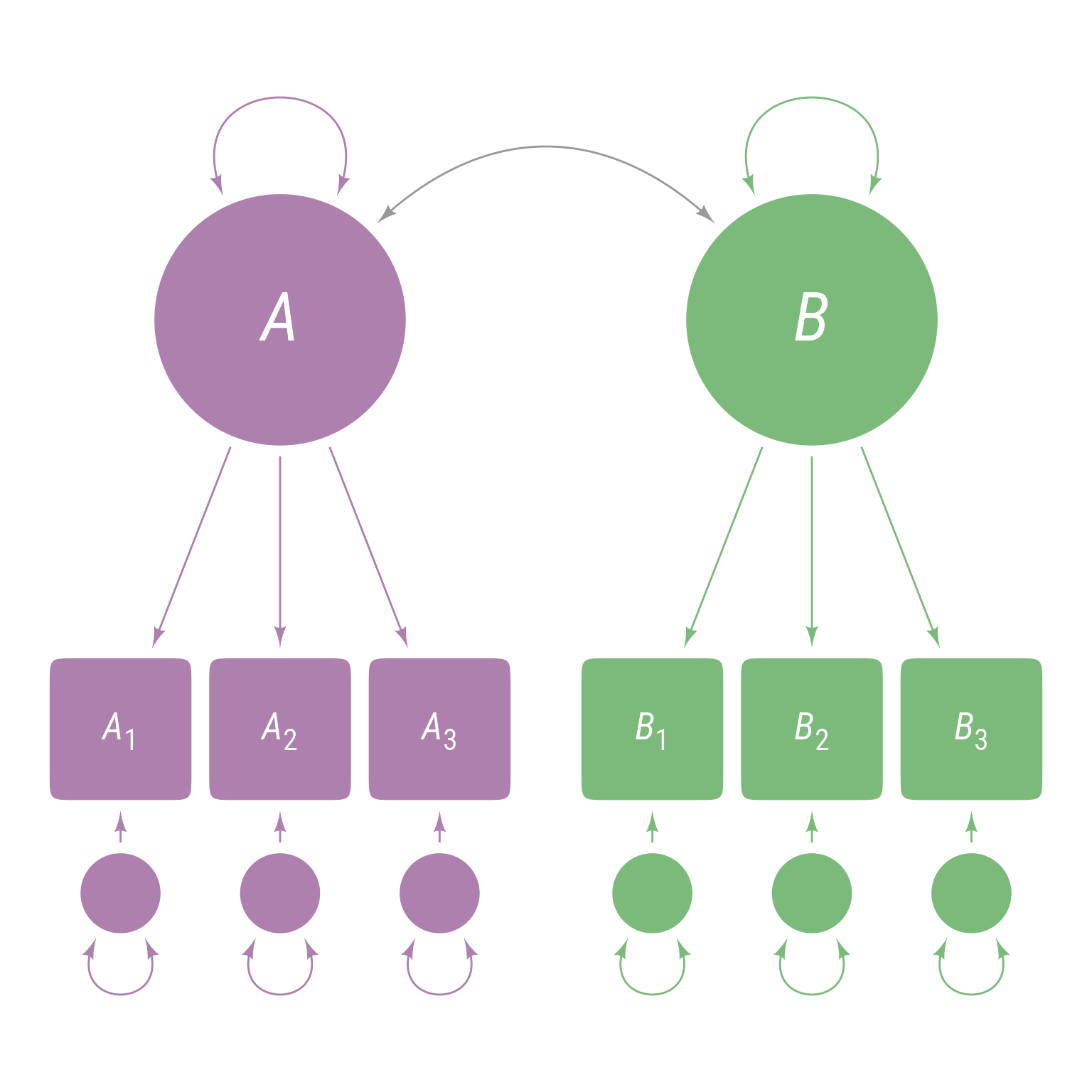
To specify that A and B are related as in Figure 5 , use the covariance operator: ~~
<- ' A =~ A1 + A2 + A3 B =~ B1 + B2 + B3 B ~~ A '
Code
+ ob_covariance (A, B, resect = 2 , color = "gray60" , looseness = .9 )
Figure 5: A latent variable model with a covariance between latent variable A and latent variable B
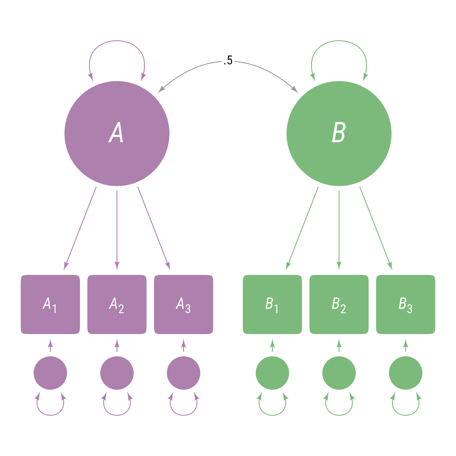
To force the covariance between A and B to be exactly 0.5 as in Figure 6 :
<- ' A =~ A1 + A2 + A3 B =~ B1 + B2 + B3 B ~~ 0.5 * A '
Code
+ ob_covariance (A, B, resect = 2 , color = "gray60" , looseness = .9 , label = ob_label (".5" , family = my_font, size = 16 ), linewidth = .5 )
Figure 6: A latent variable model with a covariance between latent variable A and latent variable B forced to equal 0
The ~~ operator is also used to specify the variance of a variable. For example, to force the variance of B to be 1 as in Figure 7 :
<- ' A =~ A1 + A2 + A3 B =~ B1 + B2 + B3 B ~~ 1 * B '
Code
+ ob_label ("1" , vB@ midpoint (), color = cB)
Figure 7: Latent variable B ’s variance is fixed to equal 1.
To specify that A1 and B1 have correlated residuals as in Figure 8 , do so like so:
<- ' A =~ A1 + A2 + A3 B =~ B1 + B2 + B3 A1 ~~ B1 '
Code
+ ob_covariance (eB3[1 ], eA3[1 ], resect = 2 , color = "gray60" , looseness = .9 , linewidth = .5 )
Figure 8: The residuals of A 1 and B 1 are allowed to covary.
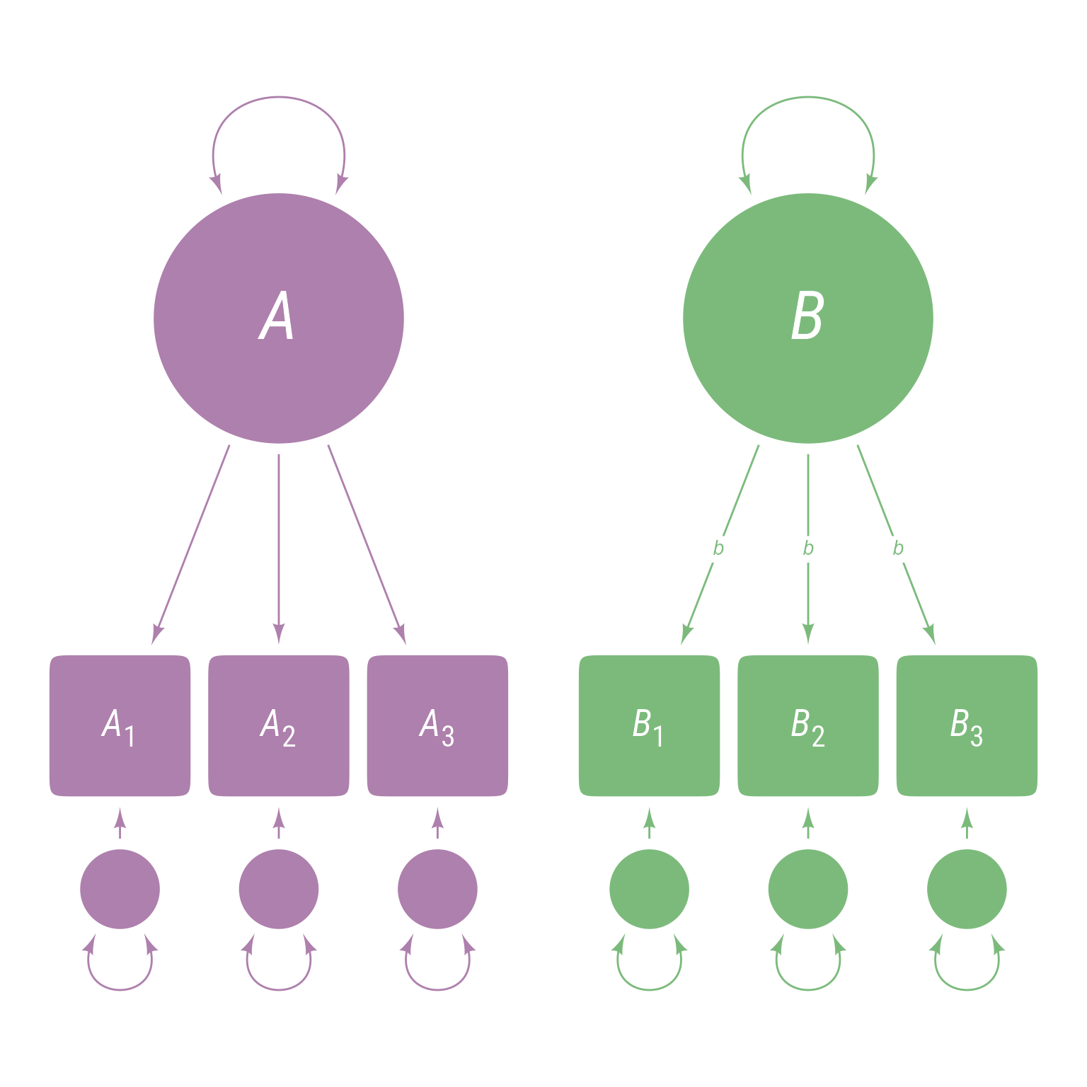
You can give any loading or covariance a variable name instead of a specific value. To force indicators to have the same loading as in Figure 9 , give them the same variable name:
<- ' A =~ A1 + A2 + A3 B =~ b * B1 + b * B2 + b * B3 '
Code
+ ob_label ("*b*" , center = load_B[2 ]@ midpoint ()@ y %>% @ line@ point_at_y ())
Figure 9: A latent variable model with all indicators of latent variable B forced to have equal loadings with value of b
Hierarchical Linear Model
Level 1 (Measurement Occasion)
Vocabulary_{ti} = b_{0i}+b_{1i}Time_{ti} +b_{2i}Time_{ti}^2+e_{ti}
Level 2 (Person)
\begin{aligned}
b_{0i}&=b_{00} + b_{01}Intervention_{i} + u_{0i}\\
b_{1i}&=b_{10} + b_{11}Intervention_{i} + u_{1i}\\
b_{2i}&=b_{20} + b_{21}Intervention_{i}
\end{aligned}
Combined Model
\begin{aligned}
Vocabulary_{ti} &=
\underbrace{b_{00} + b_{01}Intervention_{i} + u_{0i}}_{b_{0i}} +\\
&(\underbrace{b_{10} + b_{11}Intervention_{i} + u_{1i}}_{b_{1i}})Time_{ti} +\\
&(\underbrace{b_{20}+ b_{21}Intervention_{i}}_{b_{2i}})Time_{ti}^2 + e_{ti}
\end{aligned}
Code
:: tribble (~ Symbol, ~ Meaning,"$b_{00}$" , "Intercept (Predicted Vocabulary when Intervention and Time are 0)" ,"$b_{01}$" , "Slope for Intervention at Time 0" ,"$b_{10}$" , "Linear Slope for Time when Intervention and Time are 0" ,"$b_{11}$" , "Interaction of Intervention and Time at Time 0" ,"$b_{20}$" , "Quadratic Effect of Time when Intervention is 0" ,"$b_{21}$" , "Interaction of Intervention and Quadratic Effect of Time" ,"$b_{0i}$" , "Predicted Vocabulary at Time 0 for Person *i*" ,"$b_{1i}$" , "Linear Effect of Time at Time 0 for Person *i*" ,"$b_{2i}$" , "Quadratic Effect of Time for Person *i*" ,"$u_{0i}$" , "Residual for $b_{0i}$" ,"$u_{1i}$" , "Residual for $b_{1i}$" ,"$e_{ti}$" , "Residual for Person *i* at Time *t*" %>% :: kable (align = "cl" )
b_{00} Intercept (Predicted Vocabulary when Intervention and Time are 0)
b_{01} Slope for Intervention at Time 0
b_{10} Linear Slope for Time when Intervention and Time are 0
b_{11} Interaction of Intervention and Time at Time 0
b_{20} Quadratic Effect of Time when Intervention is 0
b_{21} Interaction of Intervention and Quadratic Effect of Time
b_{0i} Predicted Vocabulary at Time 0 for Person i
b_{1i} Linear Effect of Time at Time 0 for Person i
b_{2i} Quadratic Effect of Time for Person i
u_{0i} Residual for b_{0i}
u_{1i} Residual for b_{1i}
e_{ti} Residual for Person i at Time t
Table 6: Symbols and Meanings of HLM Model
Analysis
I am going straight to my hypothesized model. In a real analysis, I might have gone through the series of steps we have seen elsewhere in the course. However, I want save time so that I can show how this model is the same as the latent growth model. When I walk through all the latent growth models in sequence, I will show the comparable hierarchical linear models one at a time.
<- lmer (vocabulary ~ 1 + time * intervention + I (time ^ 2 ) * intervention + 1 + time | person_id), data = d, REML = FALSE )tab_model (m)
vocabulary
Predictors
Estimates
CI
p
(Intercept)
52.00
46.36 – 57.64
<0.001
time
10.50
9.91 – 11.09
<0.001
intervention
-0.09
-7.91 – 7.74
0.983
time^2
-1.06
-1.15 – -0.96
<0.001
time × intervention
9.14
8.33 – 9.95
<0.001
intervention × time^2
0.09
-0.05 – 0.22
0.217
Random Effects
σ2
8.99
τ00 person_id
786.64
τ11 person_id.time
2.02
ρ01 person_id
0.12
ICC
0.99
N person_id
200
Observations
1200
Marginal R2 / Conditional R2
0.381 / 0.993
We fitted a linear mixed model (estimated using ML and nloptwrap optimizer) to
predict vocabulary with time and intervention (formula: vocabulary ~ 1 + time *
intervention + I(time^2) * intervention). The model included time as random
effects (formula: ~1 + time | person_id). The model's total explanatory power
is substantial (conditional R2 = 0.99) and the part related to the fixed
effects alone (marginal R2) is of 0.38. The model's intercept, corresponding to
time = 0 and intervention = 0, is at 52.00 (95% CI [46.36, 57.64], t(1190) =
18.08, p < .001). Within this model:

  - The effect of time is statistically significant and positive (beta = 10.50,
95% CI [9.91, 11.09], t(1190) = 35.18, p < .001; Std. beta = 0.47, 95% CI
[0.46, 0.48])
  - The effect of intervention is statistically non-significant and negative
(beta = -0.09, 95% CI [-7.91, 7.74], t(1190) = -0.02, p = 0.983; Std. beta =
0.32, 95% CI [0.21, 0.43])
  - The effect of time^2 is statistically significant and negative (beta = -1.06,
95% CI [-1.15, -0.96], t(1190) = -21.10, p < .001; Std. beta = -0.08, 95% CI
[-0.09, -0.07])
  - The effect of time × intervention is statistically significant and positive
(beta = 9.14, 95% CI [8.33, 9.95], t(1190) = 22.08, p < .001; Std. beta = 0.22,
95% CI [0.21, 0.23])
  - The effect of intervention × time^2 is statistically non-significant and
positive (beta = 0.09, 95% CI [-0.05, 0.22], t(1190) = 1.24, p = 0.217; Std.
beta = 3.40e-03, 95% CI [-2.00e-03, 8.81e-03])

Standardized parameters were obtained by fitting the model on a standardized
version of the dataset. 95% Confidence Intervals (CIs) and p-values were
computed using a Wald t-distribution approximation.
Don’t be fooled by the non-significant effect of the intervention! It is a conditional effect at Time 0 —before the intervention began.
It is the interaction of time and the intervention that matters.
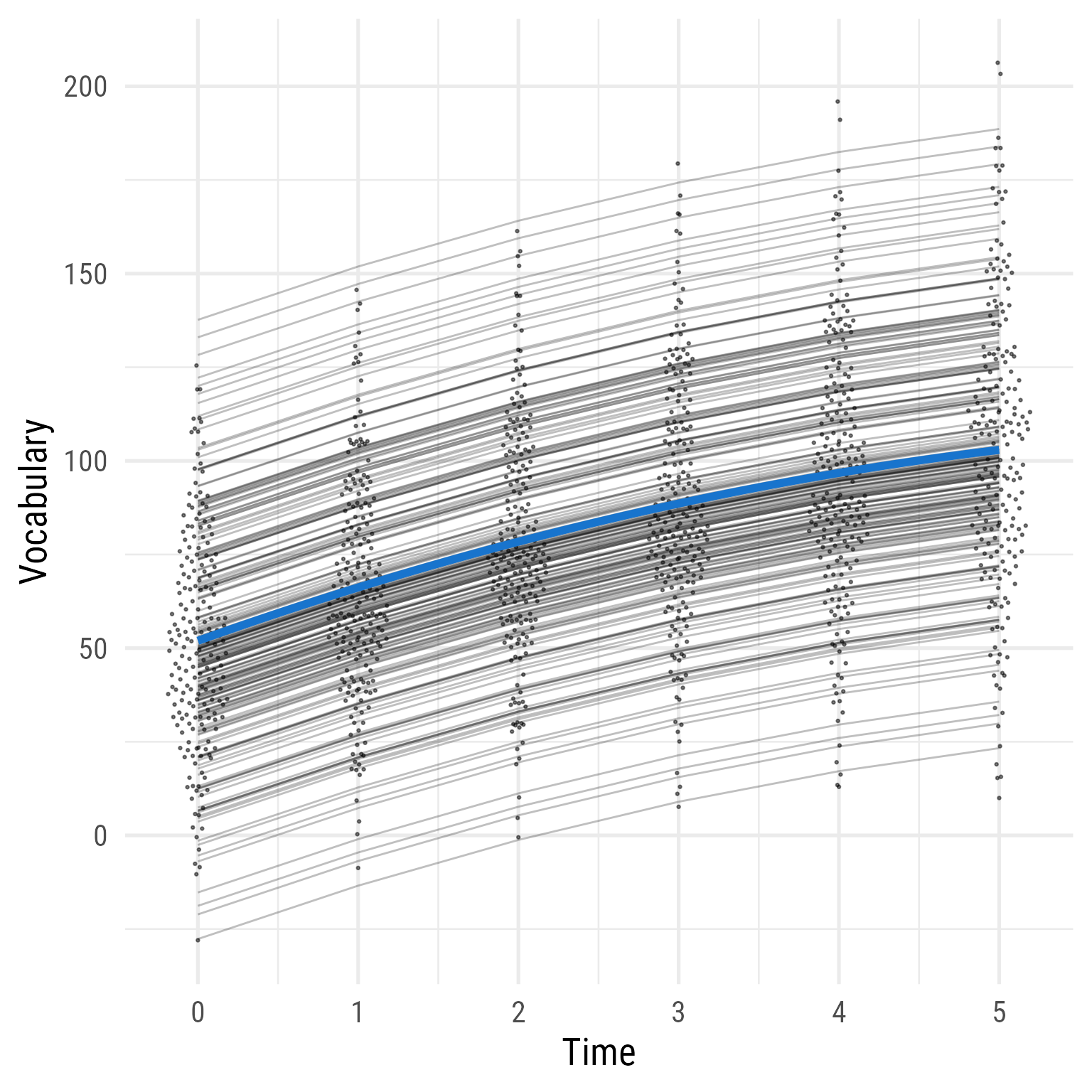
Let’s plot the model using sjPlot::plot_model:
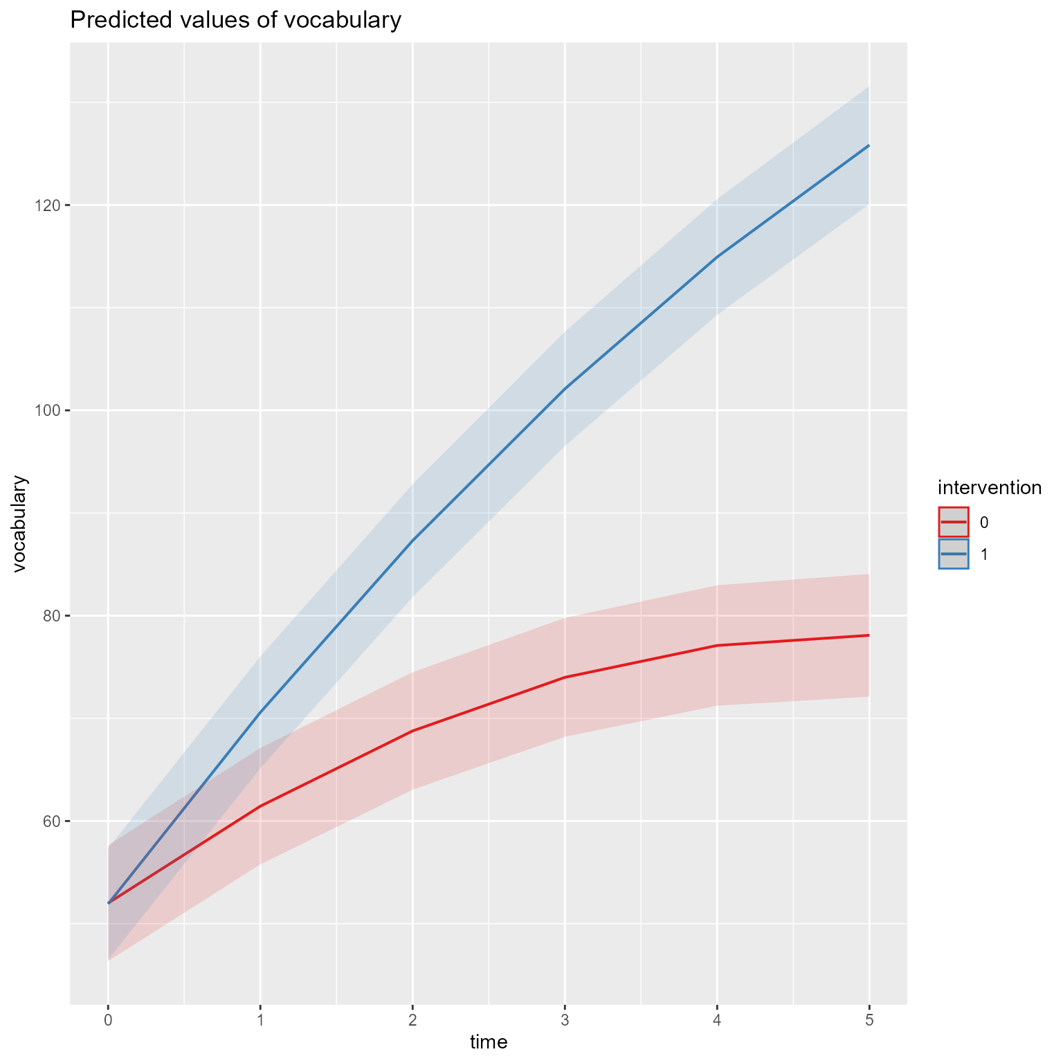
plot_model (m, type = "pred" , terms = c ("time [all]" , "intervention" ))
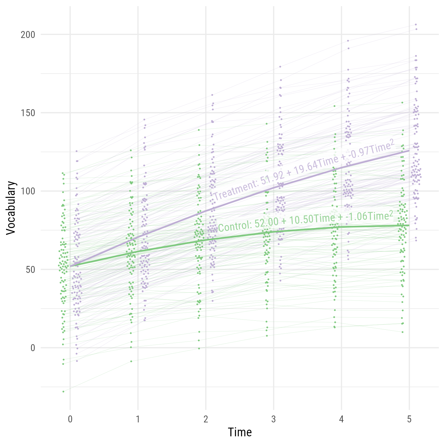
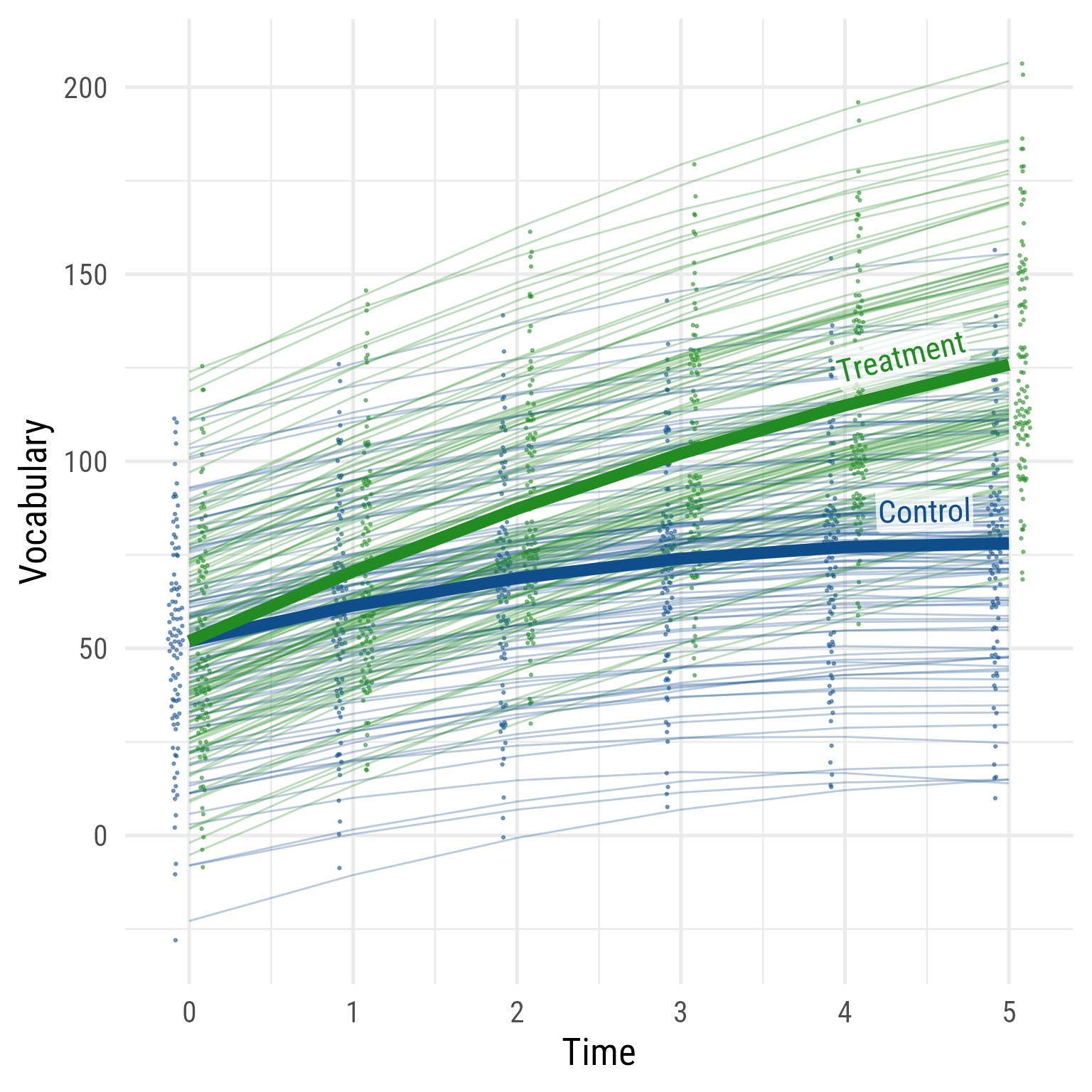
Interpretation: As hypothesized, the effect of time has diminishing returns, and the time by interaction interaction effect is evident. The two groups were comparable before the intervention, but the treatment group’s vocabulary grew faster over time. If I needed to publish a plot showing these results, it would look like Figure 10 .
Sidenote: I love the sjPlot::plot_model function. With almost no effort, I can get a plot that helps me see what is going on with my fixed effects. It used to take me so much more code to arrive at where sjPlot::plot_model lands. However, if you want a publication-worthy plot, sjPlot::plot_model tends to impose too much control. Fortunately, the same person who made sjPlot is involved with another easystats package called modelbased that allows for greater flexibility but still reduces what would otherwise be onerous coding.
Code
<- fixef (m)<- tibble (b00 = c (m_fixed["(Intercept)" ],"(Intercept)" ] + m_fixed["intervention" ]),b10 = c (m_fixed["time" ],"time" ] + m_fixed["time:intervention" ]),b20 = c (m_fixed["I(time^2)" ],"I(time^2)" ] + m_fixed["intervention:I(time^2)" ])) %>% mutate (across (.fns = \(x) formatC (x, 2 , format = "f" ))) %>% mutate (intervention = factor (c ("Control" , "Treatment" )),eq = glue:: glue ('{intervention}: {b00} + {b10}Time + {b20}Time<sup>2</sup>' )# Predicted Data <- modelbased:: estimate_relation (m, data = crossing (time = 0 : 5 , intervention = c (0 ,1 ))) %>% as_tibble () %>% mutate (intervention = factor (intervention, levels = c (0 ,1 ), labels = c ("Control" , "Treatment" ))) %>% mutate (vocabulary = Predicted, hjust = ifelse (intervention == "Treatment" , .93 , .91 )) %>% left_join (my_coefs, by = join_by (intervention)) %>% mutate (intervention = factor (intervention, levels = c (0 ,1 ), labels = c ("Control" , "Treatment" )),person_id = factor (person_id)) %>% ggplot (aes (time, vocabulary, color = intervention)) + geom_line (aes (group = person_id,x = time + (intervention == "Treatment" ) * 0.2 - 0.1 ),size = .1 , alpha = .5 ) + :: geom_quasirandom (aes (x = time + (intervention == "Treatment" ) * 0.2 - 0.1 ), width = .075 , pch = 16 , size = .75 ) + geom_line (data = d_pred,linewidth = 1 ) + geom_labelline (aes (label = eq,hjust = hjust),data = d_pred, text_only = T,alpha = .8 , size = 5 ,# linewidth = 4.25, linecolour = NA ,vjust = - 0.2 ,label.padding = unit (0 , units = "pt" ),family = "Roboto Condensed" , rich = TRUE ) + scale_x_continuous ("Time" , breaks = 0 : 5 , minor_breaks = NULL ) + scale_y_continuous ("Vocabulary" ) + theme_minimal (base_size = 16 , base_family = "Roboto Condensed" ) + theme (legend.position = "none" ) + scale_color_brewer (type = "qual" , palette = 1 )
Figure 10: The Growth of Vocabulary by Treatment Group
Latent Growth Model
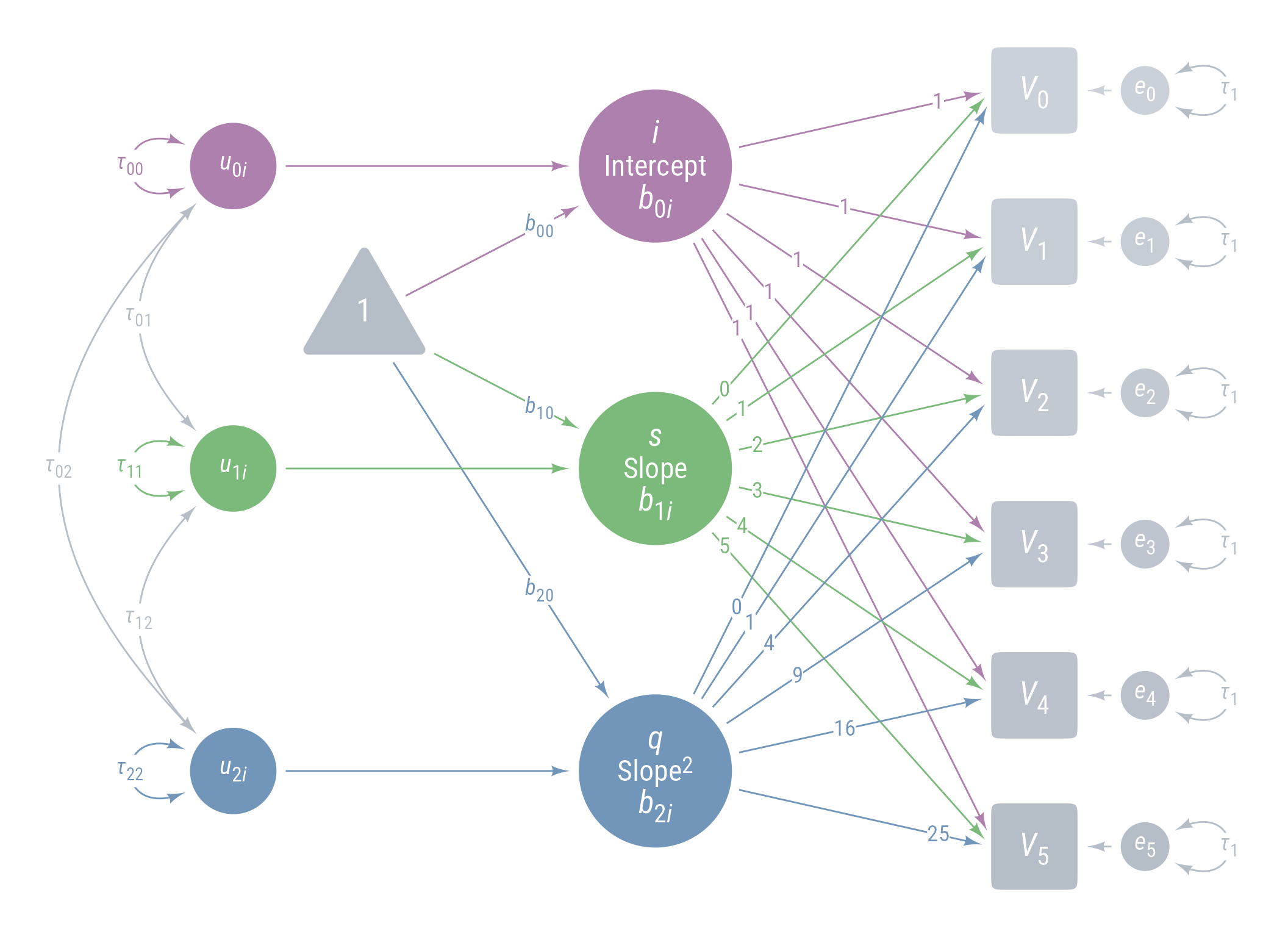
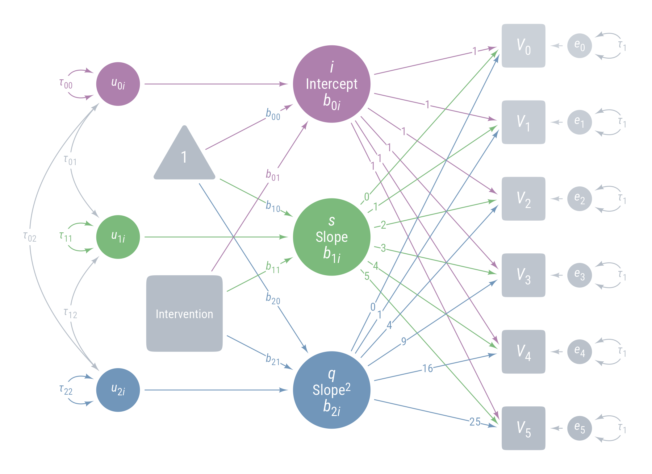
Figure 11 displays the path model for the latent growth model we are aiming for.
Code
ggdiagram (font_family = my_font, font_size = 14 ) + <- my_observed () %>% ob_array (6 ,where = "south" ,label = my_observed_label (paste0 ("*V*~" , 0 : 5 , "~" )),sep = 1.5 ,fill = class_color (cD)@ lighten (seq (0.7 , 1 , length.out = 6 ))+ my_connect (1 : 5 ],2 : 6 ],color = v@ fill[- 6 ],label = ob_label ("*r*" ,angle = 0 ,position = .4 ,size = 14 ,label.padding = margin ()resect = 1 + <- my_error (fill = v@ fill, label = my_error_label (paste0 ("*e*~" , 0 : 5 , "~" ))) %>% place (v, "right" )} + ob_variance ("right" ,label = ob_label ("*τ*~1~" ,color = cD,label.padding = margin (t = 1 )color = cD,looseness = 3.15 ,theta = degree (60 )+ my_connect (e, v, color = v@ fill) + <- my_latent (label = my_latent_label ("*i*<br><span style='font-size: 18pt'>Intercept</span><br>*b*~0*i*~" ,lineheight = 1 ,size = 20 %>% place (midpoint (v[1 ], v[2 ]), "left" , left)} + <- my_connect (i, v@ point_at (180 + seq (0 , - 10 , - 2 )))} + <- my_latent (label = my_latent_label ("*s*<br><span style='font-size: 18pt'>Slope</span><br>*b*~1*i*~" ,lineheight = 1 ,size = 20 fill = cB%>% place (midpoint (v[3 ], v[4 ]), "left" , left)} + <- my_connect (s, v@ point_at ("west" ), color = cB)} + <- my_latent (label = my_latent_label ("*q*<br><span style='font-size: 18pt'>Slope^2^</span><br>*b*~2*i*~" ,lineheight = 1 ,size = 20 fill = cC%>% place (midpoint (v[5 ], v[6 ]), "left" , left)} + <- my_connect (q, v@ point_at (180 + seq (10 , 0 , - 2 )), color = cC)} + ob_label (1 ,center = map_ob (li, \(x) intersection (x, ls[1 ]@ nudge (y = 1.1 ))),label.padding = margin (1 , 0 , 0 , 0 ),color = cA+ ob_label (0 : 5 ,center = map_ob (ls, \(x) intersection (ob_circle (s@ center, radius = s@ radius + .65 )label.padding = margin (1 , 0 , 0 , 0 ),color = cB+ ob_label ((0 : 5 )^ 2 ,center = map_ob (lq, \(x) intersection (x, ls[6 ]@ nudge (y = - 1.1 ))),label.padding = margin (1 , 0 , 0 , 0 ),color = cC+ <- my_error (radius = 1 , label = my_error_label ("*u*~0*i*~" )) %>% place (i, "left" , left)} + <- my_error (radius = 1 ,label = my_error_label ("*u*~1*i*~" ),fill = cB) %>% place (s, "left" , left)} + <- my_error (radius = 1 ,label = my_error_label ("*u*~2*i*~" ),fill = cC) %>% place (q, "left" , left)} + my_connect (u_0i, i) + my_connect (u_1i, s, color = cB) + my_connect (u_2i, q, color = cC) + <- ob_intercept (intersection (connect (u_0i, s), connect (u_1i, i)) + ob_point (- 1.85 , 0 ),width = 3 ,fill = cD,color = NA ,vertex_radius = .004 ,label = my_observed_label ("1" , vjust = .4 )+ <- bind (c (my_connect (t1, i),my_connect (t1, s, color = cB),my_connect (t1, q, color = cC)+ <- my_observed (intersection (connect (u_2i, s), connect (u_1i, q)) + ob_point (- 1.85 , 0 ),a = 1.75 ,b = 1.75 ,fill = cD,label = my_observed_label ("Intervention" , size = 15 )+ <- my_connect (intervention, bind (c (i, s, q)), color = my_colors)} + <- ob_segment (my_connect (u_0i, i)@ midpoint (.87 ),my_connect (u_2i, q)@ midpoint (.87 ))<- ob_label (paste0 ("*b*~" , 0 : 2 , "0~" ),intersection (lt0, vl),label.padding = margin (2 ),color = my_colors+ ob_label (paste0 ("*b*~" , 0 : 2 , "1~" ),intersection (lt1, vl),label.padding = margin (2 ),color = my_colors+ ob_variance (bind (c (u_0i, u_1i, u_2i)),where = "west" ,color = my_colors,looseness = 1.75 ,label = ob_label (paste0 ("*τ*~" , 0 : 2 , 0 : 2 , "~" ), color = my_colors)+ ob_covariance (bind (c (u_1i, u_2i, u_2i)),bind (c (u_0i, u_0i, u_1i)),color = cD,label = ob_label (paste0 ("*τ*~" , c (0 , 0 , 1 ), c (1 , 2 , 2 ), "~" ), color = cD))
Figure 11: Path Diagram Latent Growth Model
Restructure from Long to Wide Data
SEM analyses usually need wide data with each participant’s data on 1 row. We learned how to do so in a previous tutorial .
Use the pivot_widerd is restructured to look like this:
# A tibble: 200 × 8
   person_id intervention voc_0 voc_1 voc_2 voc_3 voc_4 voc_5
       <dbl>        <dbl> <dbl> <dbl> <dbl> <dbl> <dbl> <dbl>
 1         1            0  31.3  38.6  51.2  54.9  50.6  55.3
 2         2            0  94.1 100.  114.  119.  123.  125.
 3         3            0  57.0  66.5  73.6  80.9  88.2  93.1
 4         4            0  60.3  70.2  78.9  78.9  78.4  79.0
 5         5            0  32.6  39.1  47.3  48.1  51.1  48.3
 6         6            1  88.6 105.  120.  141.  160.  169.
 7         7            0  65.6  72.4  76.8  83.3  86.3  87.0
 8         8            0  35.9  41.7  57.4  64.8  64.1  73.1
 9         9            1  71.7  78.9  97.4 105.  121.  126.
10        10            1  75.9  85.0 106.  119.  132.  142.
# ℹ 190 more rows
See if you can figure out how to restructure the data using pivot_wider. If it takes more than a minute or two, check out the hints.
Call the new data frame d_wide.
Set the values parameter equal to vocabulary.
values = vocabulary
The names come from time.
names = time
Specify voc_ as the names prefix.
names_prefix = "voc_"
Here is how I would do it:
<- d %>% pivot_wider (names_from = time, values_from = vocabulary, names_prefix = "voc_" )
Model Specification
In general, setting up a latent growth curve model requires much more typing than the corresponding hierarchical linear model. In this model, for all this extra work we get nothing that we did not already have. However, the latent growth modeling approach is extremely flexible, particularly with respect to modeling the simultaneous effects of many other variables. In more complex models, we can evaluate hypotheses that are difficult, if not impossible, in hierarchical linear models.
Note that intercepts are symbolized with the symbol 1 when it is alone or precided by a coefficient (e.g., b_00 ~ 1)
<- " # Intercept i =~ 1 * voc_0 + 1 * voc_1 + 1 * voc_2 + 1 * voc_3 + 1 * voc_4 + 1 * voc_5 # Linear slope of time s =~ 0 * voc_0 + 1 * voc_1 + 2 * voc_2 + 3 * voc_3 + 4 * voc_4 + 5 * voc_5 # Acceleration effect of time (quadratic effect) q =~ 0 * voc_0 + 1 * voc_1 + 4 * voc_2 + 9 * voc_3 + 16 * voc_4 + 25 * voc_5 # Predicting intercept, slope, and quadratic effects i ~ b_00 * 1 + b_01 * intervention s ~ b_10 * 1 + b_11 * intervention q ~ b_20 * 1 + b_21 * intervention # Variances and covariances i ~~ tau_00 * i + tau_01 * s s ~~ tau_11 * s q ~~ 0 * q + 0 * s + 0 * i voc_0 ~~ e * voc_0 voc_1 ~~ e * voc_1 voc_2 ~~ e * voc_2 voc_3 ~~ e * voc_3 voc_4 ~~ e * voc_4 voc_5 ~~ e * voc_5 "
In the hierarchical model, we did not make b_{2i} (the quadratic effect of time) random. Thus, we will set the \tau_{22} variance to 0, and also the covariances involving u_{2i} residual (i.e., \tau_{02} and \tau_{12} ).
You can see from the summary output that the parameters are same as before.
<- growth (latent_model, data = d_wide)summary (fit_latentgrowth, fit.measures = T, standardized = T)
lavaan 0.6-19 ended normally after 111 iterations

  Estimator                                         ML
  Optimization method                           NLMINB
  Number of model parameters                        15
  Number of equality constraints                     5

  Number of observations                           200

Model Test User Model:

  Test statistic                                20.473
  Degrees of freedom                                23
  P-value (Chi-square)                           0.613

Model Test Baseline Model:

  Test statistic                              4123.548
  Degrees of freedom                                21
  P-value                                        0.000

User Model versus Baseline Model:

  Comparative Fit Index (CFI)                    1.000
  Tucker-Lewis Index (TLI)                       1.001

Loglikelihood and Information Criteria:

  Loglikelihood user model (H0)              -3806.202
  Loglikelihood unrestricted model (H1)      -3795.966

  Akaike (AIC)                                7632.405
  Bayesian (BIC)                              7665.388
  Sample-size adjusted Bayesian (SABIC)       7633.707

Root Mean Square Error of Approximation:

  RMSEA                                          0.000
  90 Percent confidence interval - lower         0.000
  90 Percent confidence interval - upper         0.051
  P-value H_0: RMSEA <= 0.050                    0.947
  P-value H_0: RMSEA >= 0.080                    0.001

Standardized Root Mean Square Residual:

  SRMR                                           0.006

Parameter Estimates:

  Standard errors                             Standard
  Information                                 Expected
  Information saturated (h1) model          Structured

Latent Variables:
                   Estimate  Std.Err  z-value  P(>|z|)   Std.lv  Std.all
  i =~
    voc_0             1.000                              28.047    0.994
    voc_1             1.000                              28.047    0.975
    voc_2             1.000                              28.047    0.931
    voc_3             1.000                              28.047    0.870
    voc_4             1.000                              28.047    0.802
    voc_5             1.000                              28.047    0.734
  s =~
    voc_0             0.000                               0.000    0.000
    voc_1             1.000                               4.781    0.166
    voc_2             2.000                               9.563    0.317
    voc_3             3.000                              14.344    0.445
    voc_4             4.000                              19.126    0.547
    voc_5             5.000                              23.907    0.625
  q =~
    voc_0             0.000                               0.000    0.000
    voc_1             1.000                               0.043    0.001
    voc_2             4.000                               0.171    0.006
    voc_3             9.000                               0.386    0.012
    voc_4            16.000                               0.686    0.020
    voc_5            25.000                               1.072    0.028

Regressions:
                   Estimate  Std.Err  z-value  P(>|z|)   Std.lv  Std.all
  i ~
    intrvnt (b_01)   -0.086    3.988   -0.022    0.983   -0.003   -0.002
  s ~
    intrvnt (b_11)    9.138    0.414   22.079    0.000    1.911    0.955
  q ~
    intrvnt (b_21)    0.086    0.069    1.236    0.217    2.002    1.000

Covariances:
                   Estimate  Std.Err  z-value  P(>|z|)   Std.lv  Std.all
 .i ~~
   .s       (t_01)    4.602    3.175    1.449    0.147    0.115    0.115
 .s ~~
   .q                 0.000                                 NaN      NaN
 .i ~~
   .q                 0.000                                 NaN      NaN

Intercepts:
                   Estimate  Std.Err  z-value  P(>|z|)   Std.lv  Std.all
   .i       (b_00)   52.002    2.876   18.082    0.000    1.854    1.854
   .s       (b_10)   10.500    0.298   35.181    0.000    2.196    2.196
   .q       (b_20)   -1.056    0.050  -21.097    0.000  -24.647  -24.647

Variances:
                   Estimate  Std.Err  z-value  P(>|z|)   Std.lv  Std.all
   .i       (t_00)  786.620   79.133    9.940    0.000    1.000    1.000
   .s       (t_11)    2.019    0.255    7.932    0.000    0.088    0.088
   .q                 0.000                               0.000    0.000
   .voc_0      (e)    8.987    0.449   20.000    0.000    8.987    0.011
   .voc_1      (e)    8.987    0.449   20.000    0.000    8.987    0.011
   .voc_2      (e)    8.987    0.449   20.000    0.000    8.987    0.010
   .voc_3      (e)    8.987    0.449   20.000    0.000    8.987    0.009
   .voc_4      (e)    8.987    0.449   20.000    0.000    8.987    0.007
   .voc_5      (e)    8.987    0.449   20.000    0.000    8.987    0.006
Notice that we went straight to the final model. We could have done a sequence of steps identical to the hierarchical linear model.
I will show the sequence of models and compare them.
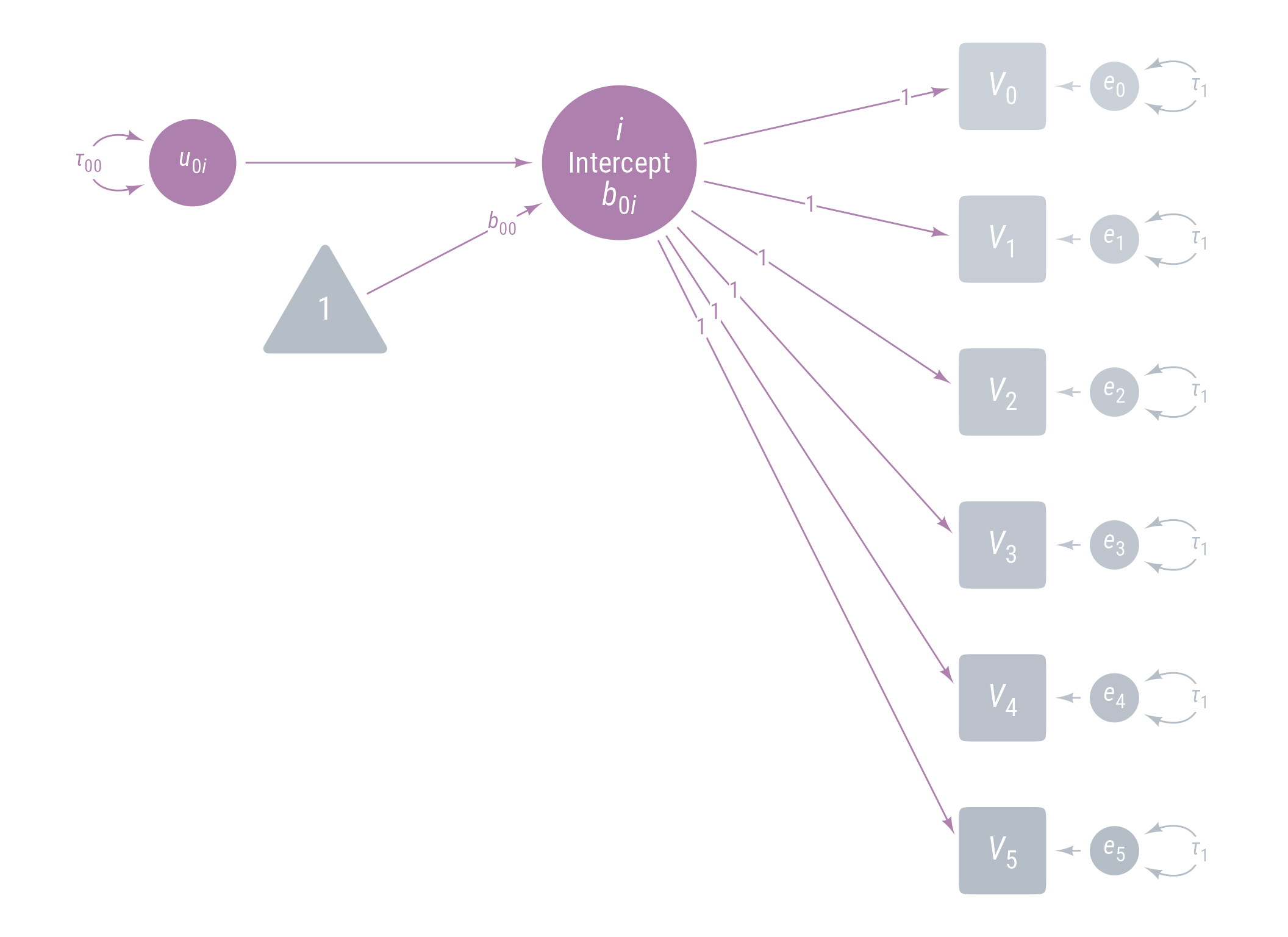
Model 0: Random Intercepts
Code
<- ggdiagram (font_family = my_font, font_size = 14 ) + <- my_observed () %>% ob_array (6 ,where = "south" ,label = my_observed_label (paste0 ("*V*~" , 0 : 5 , "~" )),sep = 1.5 ,fill = class_color (cD)@ lighten (seq (0.7 , 1 , length.out = 6 ))+ <- my_error (fill = v@ fill, label = my_error_label (paste0 ("*e*~" , 0 : 5 , "~" ))) %>% place (v, "right" )} + ob_variance ("right" ,label = ob_label ("*τ*~1~" ,color = cD,label.padding = margin (t = 1 )color = cD,looseness = 3.15 ,theta = degree (60 )+ my_connect (e, v, color = v@ fill) + <- my_latent (label = my_latent_label ("*i*<br><span style='font-size: 18pt'>Intercept</span><br>*b*~0*i*~" ,lineheight = 1 ,size = 20 %>% place (midpoint (v[1 ], v[2 ]), "left" , left)} + <- my_connect (i, v@ point_at (180 + seq (0 , - 10 , - 2 )))} + ob_label (1 ,center = map_ob (li, \(x) intersection (x, ls[1 ]@ nudge (y = 1.1 ))),label.padding = margin (1 , 0 , 0 , 0 ),color = cA+ <- my_error (radius = 1 , label = my_error_label ("*u*~0*i*~" )) %>% place (i, "left" , left)} + my_connect (u_0i, i) + <- ob_intercept (intersection (connect (u_0i, s), connect (u_1i, i)) + ob_point (- 1.85 , 0 ),width = 3 ,fill = cD,color = NA ,vertex_radius = .004 ,label = my_observed_label ("1" , vjust = .4 )+ <- my_connect (t1, i)} + <- ob_segment (my_connect (u_0i, i)@ midpoint (.87 ),my_connect (u_2i, q)@ midpoint (.87 ), alpha = 0 )} + ob_label ("*b*~00~" ,intersection (b00, vl),label.padding = margin (2 ),color = cA+ ob_variance (where = "west" ,color = cA,looseness = 1.75 ,label = ob_label (paste0 ("*τ*~00~" ), color = cA))
Figure 12: Path Diagram for Model 0
As usual, we start with a simple model with random intercepts. Time is not yet included in the model. The latent variable i has a mean of b_{00} and a variance of \tau_{00} . The variances of error terms for each observed variable are constrained to be equal (\tau_1) . The intercepts of the observed variables are not modeled here, so they are assumbed to be 0.
<- ' # Intercept i =~ 1 * voc_0 + 1 * voc_1 + 1 * voc_2 + 1 * voc_3 + 1 * voc_4 + 1 * voc_5 # Intercept, slope, and quadratic effects i ~ b_00 * 1 # Variances and covariances i ~~ tau_00 * i voc_0 ~~ e * voc_0 voc_1 ~~ e * voc_1 voc_2 ~~ e * voc_2 voc_3 ~~ e * voc_3 voc_4 ~~ e * voc_4 voc_5 ~~ e * voc_5 ' <- growth (m_0, data = d_wide)# The standard way to get output from lavaan summary (fit_0, fit.measures = T, standardized = T)
lavaan 0.6-19 ended normally after 18 iterations

  Estimator                                         ML
  Optimization method                           NLMINB
  Number of model parameters                         8
  Number of equality constraints                     5

  Number of observations                           200

Model Test User Model:

  Test statistic                              3228.267
  Degrees of freedom                                24
  P-value (Chi-square)                           0.000

Model Test Baseline Model:

  Test statistic                              3659.200
  Degrees of freedom                                15
  P-value                                        0.000

User Model versus Baseline Model:

  Comparative Fit Index (CFI)                    0.121
  Tucker-Lewis Index (TLI)                       0.450

Loglikelihood and Information Criteria:

  Loglikelihood user model (H0)              -5642.273
  Loglikelihood unrestricted model (H1)      -4028.140

  Akaike (AIC)                               11290.547
  Bayesian (BIC)                             11300.442
  Sample-size adjusted Bayesian (SABIC)      11290.938

Root Mean Square Error of Approximation:

  RMSEA                                          0.817
  90 Percent confidence interval - lower         0.793
  90 Percent confidence interval - upper         0.841
  P-value H_0: RMSEA <= 0.050                    0.000
  P-value H_0: RMSEA >= 0.080                    1.000

Standardized Root Mean Square Residual:

  SRMR                                           0.357

Parameter Estimates:

  Standard errors                             Standard
  Information                                 Expected
  Information saturated (h1) model          Structured

Latent Variables:
                   Estimate  Std.Err  z-value  P(>|z|)   Std.lv  Std.all
  i =~
    voc_0             1.000                              29.736    0.809
    voc_1             1.000                              29.736    0.809
    voc_2             1.000                              29.736    0.809
    voc_3             1.000                              29.736    0.809
    voc_4             1.000                              29.736    0.809
    voc_5             1.000                              29.736    0.809

Intercepts:
                   Estimate  Std.Err  z-value  P(>|z|)   Std.lv  Std.all
    i       (b_00)   80.811    2.193   36.844    0.000    2.718    2.718

Variances:
                   Estimate  Std.Err  z-value  P(>|z|)   Std.lv  Std.all
    i       (t_00)  884.245   96.275    9.185    0.000    1.000    1.000
   .voc_0      (e)  467.273   20.897   22.361    0.000  467.273    0.346
   .voc_1      (e)  467.273   20.897   22.361    0.000  467.273    0.346
   .voc_2      (e)  467.273   20.897   22.361    0.000  467.273    0.346
   .voc_3      (e)  467.273   20.897   22.361    0.000  467.273    0.346
   .voc_4      (e)  467.273   20.897   22.361    0.000  467.273    0.346
   .voc_5      (e)  467.273   20.897   22.361    0.000  467.273    0.346
# The easystats way parameters (fit_0, component = "all" )
# Loading

Link       | Coefficient |   SE |       95% CI |      p
-------------------------------------------------------
i =~ voc_0 |        1.00 | 0.00 | [1.00, 1.00] | < .001
i =~ voc_1 |        1.00 | 0.00 | [1.00, 1.00] | < .001
i =~ voc_2 |        1.00 | 0.00 | [1.00, 1.00] | < .001
i =~ voc_3 |        1.00 | 0.00 | [1.00, 1.00] | < .001
i =~ voc_4 |        1.00 | 0.00 | [1.00, 1.00] | < .001
i =~ voc_5 |        1.00 | 0.00 | [1.00, 1.00] | < .001

# Mean

Link         | Coefficient |   SE |         95% CI |     z |      p
-------------------------------------------------------------------
i ~1  (b_00) |       80.81 | 2.19 | [76.51, 85.11] | 36.84 | < .001
voc_0 ~1     |        0.00 | 0.00 | [ 0.00,  0.00] |       | < .001
voc_1 ~1     |        0.00 | 0.00 | [ 0.00,  0.00] |       | < .001
voc_2 ~1     |        0.00 | 0.00 | [ 0.00,  0.00] |       | < .001
voc_3 ~1     |        0.00 | 0.00 | [ 0.00,  0.00] |       | < .001
voc_4 ~1     |        0.00 | 0.00 | [ 0.00,  0.00] |       | < .001
voc_5 ~1     |        0.00 | 0.00 | [ 0.00,  0.00] |       | < .001

# Variance

Link               | Coefficient |    SE |            95% CI |     z |      p
-----------------------------------------------------------------------------
i ~~ i (tau_00)    |      884.25 | 96.28 | [695.55, 1072.94] |  9.18 | < .001
voc_0 ~~ voc_0 (e) |      467.27 | 20.90 | [426.32,  508.23] | 22.36 | < .001
voc_1 ~~ voc_1 (e) |      467.27 | 20.90 | [426.32,  508.23] | 22.36 | < .001
voc_2 ~~ voc_2 (e) |      467.27 | 20.90 | [426.32,  508.23] | 22.36 | < .001
voc_3 ~~ voc_3 (e) |      467.27 | 20.90 | [426.32,  508.23] | 22.36 | < .001
voc_4 ~~ voc_4 (e) |      467.27 | 20.90 | [426.32,  508.23] | 22.36 | < .001
voc_5 ~~ voc_5 (e) |      467.27 | 20.90 | [426.32,  508.23] | 22.36 | < .001
# There are many fit indices. https://easystats.github.io/performance/reference/model_performance.lavaan.html # Here are some common indices: <- c ("CFI" , "NNFI" , "AGFI" , "RMSEA" , "AIC" , "BIC" )performance (fit_0, metrics = my_metrics)
# Indices of model performance

CFI   |  NNFI |  AGFI | RMSEA |       AIC |       BIC
-----------------------------------------------------
0.121 | 0.450 | 0.426 | 0.817 | 11290.547 | 11300.442
Not surprisingly, the fit statistics of our null model indicate poor fit. The CFI (Comparative Fit Index), NNFI (Non-Normed Fit Index), and AGFI (Adjusted Goodness of Fit) approach 1 when the fit is good. There are no absolute standards for these fit indices, and good values can vary from model to model, but in general look for values better than .90. The RMSEA (Root Mean Squared Error of Approximation) approaches 0 when fit is good. Again, there is no absolute standard for the RMSEA but in general look for values below .10 and be pleased when values are below .05.
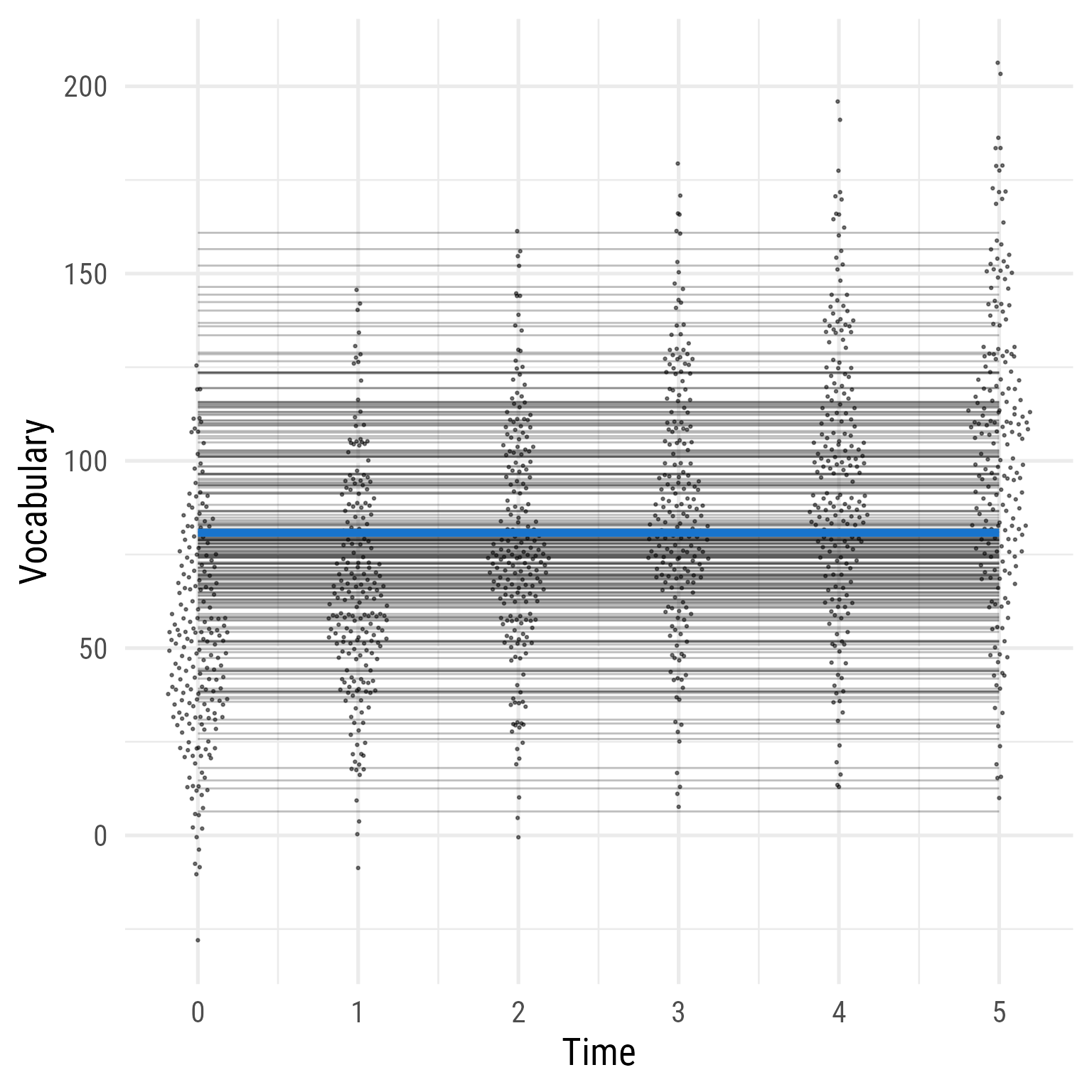
The reason that the data fit poorly can be seen clearly in Figure 13 . Although vocabulary clearly increases over time, Model 0 constrains the prediction to not grow—to be the same for each person across time.
Code
<- function (fit) {lavPredict (fit, type = "ov" ) %>% as_tibble () %>% mutate (across (everything (), .fns = as.numeric)) %>% mutate (person_id = dplyr:: row_number ()) %>% pivot_longer (starts_with ("voc_" ),values_to = "vocabulary" ,names_to = "time" ,names_prefix = "voc_" ,names_transform = list (time = as.integer)%>% mutate (person_id = factor (person_id) %>% fct_reorder (vocabulary))ggplot (d, aes (time, vocabulary)) + :: geom_quasirandom (width = .2 , size = .5 , alpha = .5 ) + geom_line (data = predict (fit_0) %>% as_tibble () %>% mutate (across (everything (), .fns = as.numeric)) %>% mutate (person_id = dplyr:: row_number ()) %>% crossing (time = 0 : 5 ) %>% mutate (vocabulary = i ),aes (group = person_id),alpha = .25 ,+ stat_function (data = tibble (x = 0 : 5 ),geom = "line" ,fun = \(x) coef (fit_0)["b_00" ] ,inherit.aes = F,color = "dodgerblue3" ,linewidth = 2 + theme_minimal (base_size = 20 , base_family = my_font) + labs (x = "Time" , y = "Vocabulary" )
Figure 13: Model 0: Random Intercepts)
As seen in Table 7 , the various parameters of the analogous hierarchical linear model are nearly identical—if maximum likelihood is used instead of restricted maximum likelihood (i.e., REML = FALSE)
lmer (vocabulary ~ 1 + (1 | person_id), data = d, REML = FALSE ) %>% tab_model ()
vocabulary
Predictors
Estimates
CI
p
(Intercept)
80.81
76.51 – 85.11
<0.001
Random Effects
σ2
467.27
τ00 person_id
884.25
ICC
0.65
N person_id
200
Observations
1200
Marginal R2 / Conditional R2
0.000 / 0.654
Table 7: HLM Model Analogous to Model 0
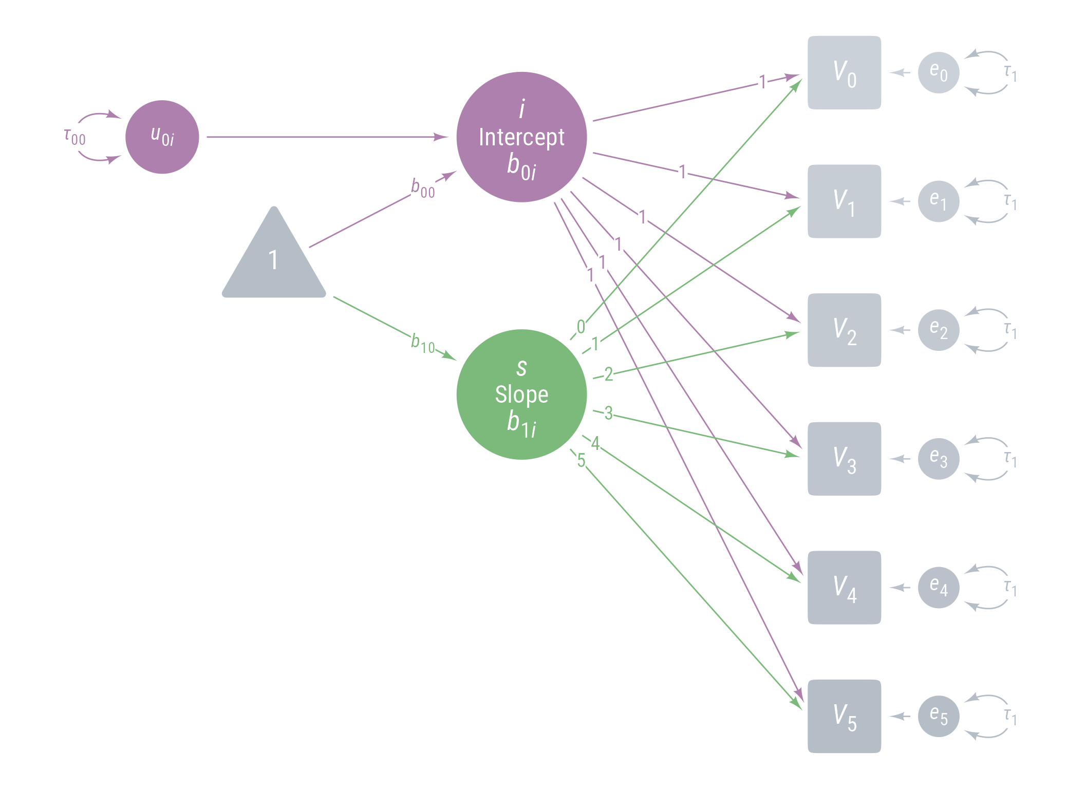
Model 1: Model 0 + Fixed Linear Effect of Time
Code
<- pd0 + <- my_latent (label = my_latent_label ("*s*<br><span style='font-size: 18pt'>Slope</span><br>*b*~1*i*~" ,lineheight = 1 ,size = 20 fill = cB%>% place (midpoint (v[3 ], v[4 ]), "left" , left)} + <- my_connect (s, v@ point_at ("west" ), color = cB)} + <- my_connect (t1, s, color = cB)} + ob_label ("*b*~10~" ,intersection (b10, vl),label.padding = margin (2 ),color = cB+ ob_label (0 : 5 ,center = map_ob (ls, \(x) intersection (ob_circle (s@ center, radius = s@ radius + .65 )label.padding = margin (1 , 0 , 0 , 0 ),color = cB
Figure 14: Path Diagram for Model 1
We add a fixed slope for time (latent variable s ), setting the residual variance of s and its covariance with the intercept i to 0.
<- " # Intercept i =~ 1 * voc_0 + 1 * voc_1 + 1 * voc_2 + 1 * voc_3 + 1 * voc_4 + 1 * voc_5 # Linear slope of time s =~ 0 * voc_0 + 1 * voc_1 + 2 * voc_2 + 3 * voc_3 + 4 * voc_4 + 5 * voc_5 # Intercept, slope, and quadratic effects i ~ b_00 * 1 s ~ b_10 * 1 # Variances and covariances i ~~ tau_00 * i s ~~ 0 * s + 0 * i voc_0 ~~ e * voc_0 voc_1 ~~ e * voc_1 voc_2 ~~ e * voc_2 voc_3 ~~ e * voc_3 voc_4 ~~ e * voc_4 voc_5 ~~ e * voc_5 " <- growth (m_1, data = d_wide)parameters (fit_1, component = "all" )
# Loading

Link       | Coefficient |   SE |       95% CI |      p
-------------------------------------------------------
i =~ voc_0 |        1.00 | 0.00 | [1.00, 1.00] | < .001
i =~ voc_1 |        1.00 | 0.00 | [1.00, 1.00] | < .001
i =~ voc_2 |        1.00 | 0.00 | [1.00, 1.00] | < .001
i =~ voc_3 |        1.00 | 0.00 | [1.00, 1.00] | < .001
i =~ voc_4 |        1.00 | 0.00 | [1.00, 1.00] | < .001
i =~ voc_5 |        1.00 | 0.00 | [1.00, 1.00] | < .001
s =~ voc_0 |        0.00 | 0.00 | [0.00, 0.00] | < .001
s =~ voc_1 |        1.00 | 0.00 | [1.00, 1.00] | < .001
s =~ voc_2 |        2.00 | 0.00 | [2.00, 2.00] | < .001
s =~ voc_3 |        3.00 | 0.00 | [3.00, 3.00] | < .001
s =~ voc_4 |        4.00 | 0.00 | [4.00, 4.00] | < .001
s =~ voc_5 |        5.00 | 0.00 | [5.00, 5.00] | < .001

# Mean

Link         | Coefficient |   SE |         95% CI |     z |      p
-------------------------------------------------------------------
i ~1  (b_00) |       55.33 | 2.24 | [50.95, 59.71] | 24.75 | < .001
s ~1  (b_10) |       10.19 | 0.17 | [ 9.86, 10.53] | 59.22 | < .001
voc_0 ~1     |        0.00 | 0.00 | [ 0.00,  0.00] |       | < .001
voc_1 ~1     |        0.00 | 0.00 | [ 0.00,  0.00] |       | < .001
voc_2 ~1     |        0.00 | 0.00 | [ 0.00,  0.00] |       | < .001
voc_3 ~1     |        0.00 | 0.00 | [ 0.00,  0.00] |       | < .001
voc_4 ~1     |        0.00 | 0.00 | [ 0.00,  0.00] |       | < .001
voc_5 ~1     |        0.00 | 0.00 | [ 0.00,  0.00] |       | < .001

# Variance

Link               | Coefficient |    SE |            95% CI |     z |      p
-----------------------------------------------------------------------------
i ~~ i (tau_00)    |      944.85 | 96.22 | [756.27, 1133.42] |  9.82 | < .001
s ~~ s             |        0.00 |  0.00 | [  0.00,    0.00] |       | < .001
voc_0 ~~ voc_0 (e) |      103.67 |  4.64 | [ 94.59,  112.76] | 22.36 | < .001
voc_1 ~~ voc_1 (e) |      103.67 |  4.64 | [ 94.59,  112.76] | 22.36 | < .001
voc_2 ~~ voc_2 (e) |      103.67 |  4.64 | [ 94.59,  112.76] | 22.36 | < .001
voc_3 ~~ voc_3 (e) |      103.67 |  4.64 | [ 94.59,  112.76] | 22.36 | < .001
voc_4 ~~ voc_4 (e) |      103.67 |  4.64 | [ 94.59,  112.76] | 22.36 | < .001
voc_5 ~~ voc_5 (e) |      103.67 |  4.64 | [ 94.59,  112.76] | 22.36 | < .001

# Correlation

Link   | Coefficient |   SE |       95% CI |      p
---------------------------------------------------
i ~~ s |        0.00 | 0.00 | [0.00, 0.00] | < .001
Let’s see if adding the linear effect of time improved model fit:
# Compare new model with the previous model test_likelihoodratio (fit_0, fit_1)
# Likelihood-Ratio-Test (LRT) for Model Comparison

Model |   Type | df | df_diff |    Chi2 |      p
------------------------------------------------
fit_0 | lavaan | 24 |       1 | 3228.27 | < .001
fit_1 | lavaan | 23 |         | 1722.61 |
compare_performance (fit_0, fit_1, metrics = my_metrics)
# Comparison of Model Performance Indices

Name  |  Model |   CFI |  NNFI |  AGFI | RMSEA
----------------------------------------------
fit_0 | lavaan | 0.121 | 0.450 | 0.426 | 0.817
fit_1 | lavaan | 0.534 | 0.696 | 0.726 | 0.608
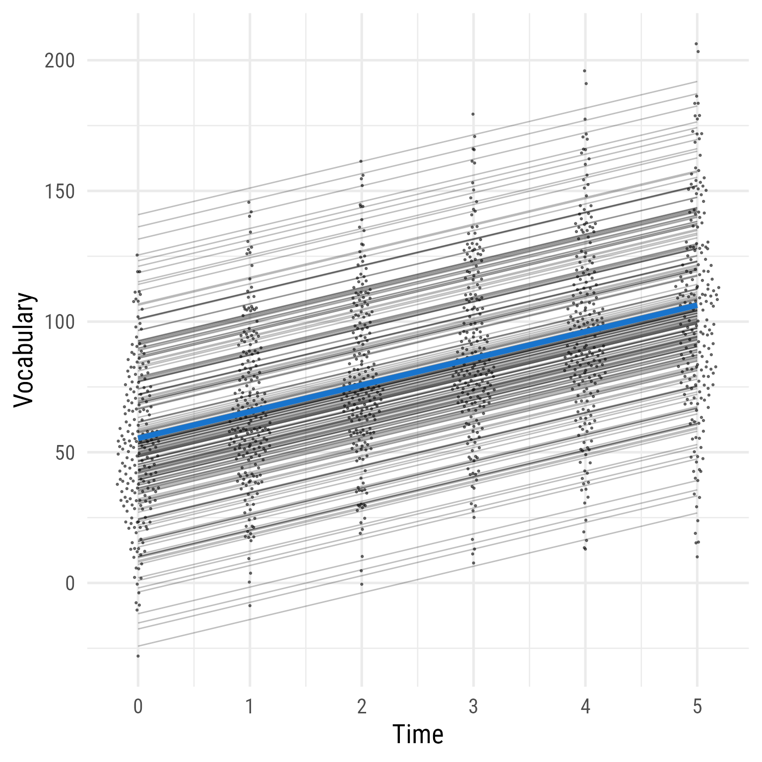
Because the p-value is significant, adding the linear effect of time improved the model fit.
Code
ggplot (d, aes (time, vocabulary)) + :: geom_quasirandom (width = .2 , size = .5 , alpha = .5 ) + geom_line (data = predict (fit_1) %>% as_tibble () %>% mutate (across (everything (), .fns = as.numeric)) %>% mutate (person_id = dplyr:: row_number ()) %>% crossing (time = 0 : 5 ) %>% mutate (vocabulary = i + s * time),aes (group = person_id),alpha = .25 ,+ stat_function (data = tibble (x = 0 : 5 ),geom = "line" ,fun = \(x) coef (fit_1)["b_00" ] + coef (fit_1)["b_10" ] * x ,inherit.aes = F,color = "dodgerblue3" ,linewidth = 2 + theme_minimal (base_size = 20 , base_family = my_font) + labs (x = "Time" , y = "Vocabulary" )
Figure 15: Model 1: Predicted Vocabulary Over Time (Model 0 + Linear Effect of Time)
As seen in Table 8 , the various parameters of the analogous hierarchical linear model are nearly identical.
lmer (vocabulary ~ 1 + time + (1 | person_id), data = d, REML = FALSE ) %>% tab_model ()
vocabulary
Predictors
Estimates
CI
p
(Intercept)
55.33
50.94 – 59.72
<0.001
time
10.19
9.85 – 10.53
<0.001
Random Effects
σ2
103.67
τ00 person_id
944.84
ICC
0.90
N person_id
200
Observations
1200
Marginal R2 / Conditional R2
0.224 / 0.923
Table 8: HLM Model Analogous to Model 1
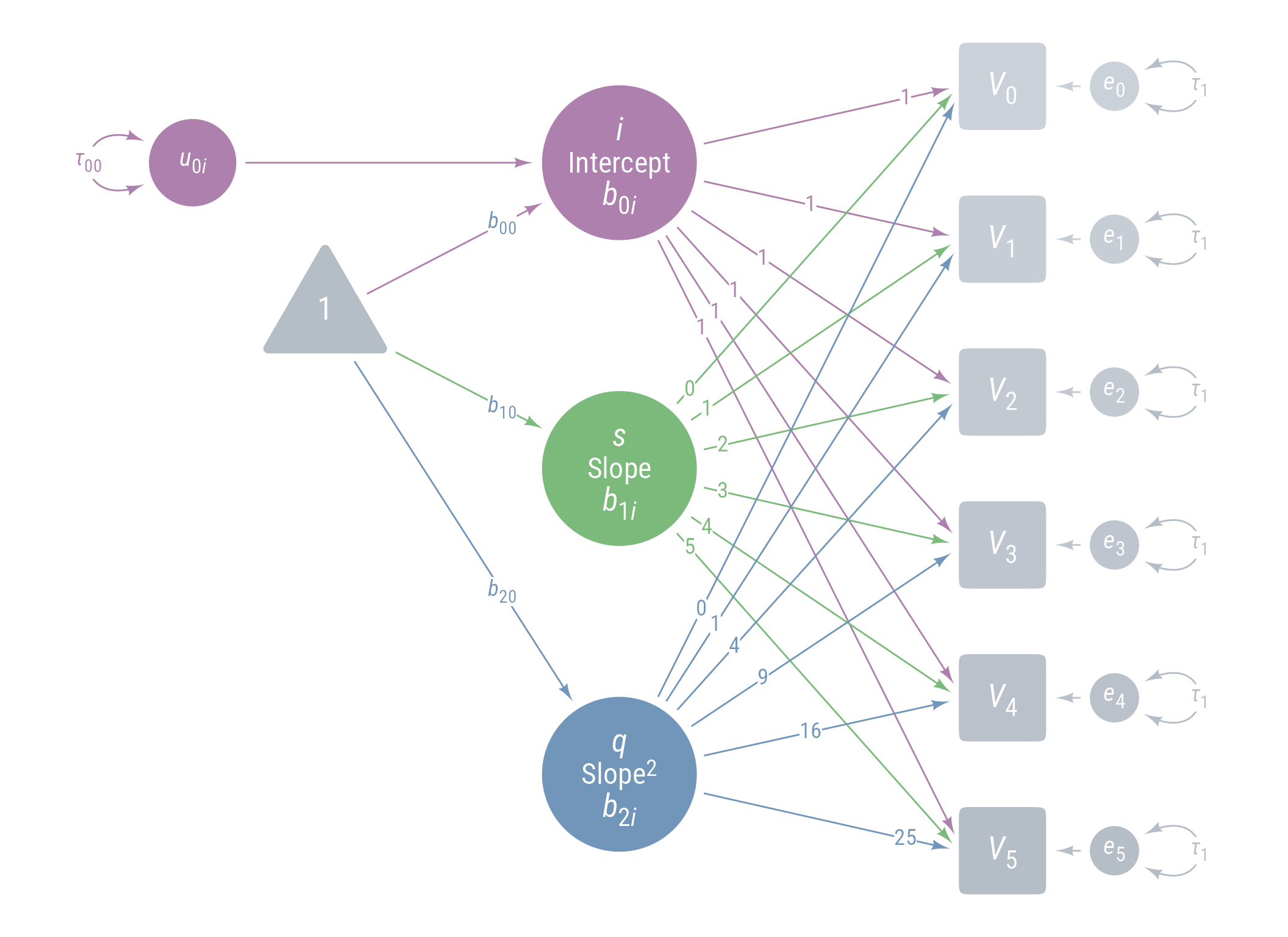
Model 2: Model 1 + Quadratic Effect of Time
Code
<- pd1 + <- my_latent (label = my_latent_label ("*q*<br><span style='font-size: 18pt'>Slope^2^</span><br>*b*~2*i*~" ,lineheight = 1 ,size = 20 fill = cC%>% place (midpoint (v[5 ], v[6 ]), "left" , left)} + <- my_connect (q, v@ point_at (180 + seq (10 , 0 , - 2 )), color = cC)} + ob_label ((0 : 5 )^ 2 ,center = map_ob (lq, \(x) intersection (x, ls[6 ]@ nudge (y = - 1.1 ))),label.padding = margin (1 , 0 , 0 , 0 ),color = cC+ <- my_connect (t1, q, color = cC)} + ob_label ("*b*~20~" ,intersection (b20, vl),label.padding = margin (2 ),color = cC
Figure 16: Path Diagram for Model 2
We set a fixed quadratic effect for time, with the residual variance set to 0.
<- " # Intercept i =~ 1 * voc_0 + 1 * voc_1 + 1 * voc_2 + 1 * voc_3 + 1 * voc_4 + 1 * voc_5 # Linear slope of time s =~ 0 * voc_0 + 1 * voc_1 + 2 * voc_2 + 3 * voc_3 + 4 * voc_4 + 5 * voc_5 # Acceleration effect of time (quadratic effect) q =~ 0 * voc_0 + 1 * voc_1 + 4 * voc_2 + 9 * voc_3 + 16 * voc_4 + 25 * voc_5 # Intercept, slope, and quadratic effects i ~ b_00 * 1 s ~ b_10 * 1 q ~ b_20 * 1 # Variances and covariances i ~~ tau_00 * i s ~~ 0 * s + 0 * i q ~~ 0 * q + 0 * s + 0 * i voc_0 ~~ e * voc_0 voc_1 ~~ e * voc_1 voc_2 ~~ e * voc_2 voc_3 ~~ e * voc_3 voc_4 ~~ e * voc_4 voc_5 ~~ e * voc_5 " <- growth (m_2, data = d_wide)parameters (fit_2, component = "all" )
# Loading

Link       | Coefficient |   SE |         95% CI |      p
---------------------------------------------------------
i =~ voc_0 |        1.00 | 0.00 | [ 1.00,  1.00] | < .001
i =~ voc_1 |        1.00 | 0.00 | [ 1.00,  1.00] | < .001
i =~ voc_2 |        1.00 | 0.00 | [ 1.00,  1.00] | < .001
i =~ voc_3 |        1.00 | 0.00 | [ 1.00,  1.00] | < .001
i =~ voc_4 |        1.00 | 0.00 | [ 1.00,  1.00] | < .001
i =~ voc_5 |        1.00 | 0.00 | [ 1.00,  1.00] | < .001
s =~ voc_0 |        0.00 | 0.00 | [ 0.00,  0.00] | < .001
s =~ voc_1 |        1.00 | 0.00 | [ 1.00,  1.00] | < .001
s =~ voc_2 |        2.00 | 0.00 | [ 2.00,  2.00] | < .001
s =~ voc_3 |        3.00 | 0.00 | [ 3.00,  3.00] | < .001
s =~ voc_4 |        4.00 | 0.00 | [ 4.00,  4.00] | < .001
s =~ voc_5 |        5.00 | 0.00 | [ 5.00,  5.00] | < .001
q =~ voc_0 |        0.00 | 0.00 | [ 0.00,  0.00] | < .001
q =~ voc_1 |        1.00 | 0.00 | [ 1.00,  1.00] | < .001
q =~ voc_2 |        4.00 | 0.00 | [ 4.00,  4.00] | < .001
q =~ voc_3 |        9.00 | 0.00 | [ 9.00,  9.00] | < .001
q =~ voc_4 |       16.00 | 0.00 | [16.00, 16.00] | < .001
q =~ voc_5 |       25.00 | 0.00 | [25.00, 25.00] | < .001

# Mean

Link         | Coefficient |   SE |         95% CI |     z |      p
-------------------------------------------------------------------
i ~1  (b_00) |       51.96 | 2.26 | [47.52, 56.39] | 22.95 | < .001
s ~1  (b_10) |       15.25 | 0.59 | [14.09, 16.41] | 25.82 | < .001
q ~1  (b_20) |       -1.01 | 0.11 | [-1.23, -0.79] | -8.92 | < .001
voc_0 ~1     |        0.00 | 0.00 | [ 0.00,  0.00] |       | < .001
voc_1 ~1     |        0.00 | 0.00 | [ 0.00,  0.00] |       | < .001
voc_2 ~1     |        0.00 | 0.00 | [ 0.00,  0.00] |       | < .001
voc_3 ~1     |        0.00 | 0.00 | [ 0.00,  0.00] |       | < .001
voc_4 ~1     |        0.00 | 0.00 | [ 0.00,  0.00] |       | < .001
voc_5 ~1     |        0.00 | 0.00 | [ 0.00,  0.00] |       | < .001

# Variance

Link               | Coefficient |    SE |            95% CI |     z |      p
-----------------------------------------------------------------------------
i ~~ i (tau_00)    |      946.11 | 96.21 | [757.54, 1134.69] |  9.83 | < .001
s ~~ s             |        0.00 |  0.00 | [  0.00,    0.00] |       | < .001
q ~~ q             |        0.00 |  0.00 | [  0.00,    0.00] |       | < .001
voc_0 ~~ voc_0 (e) |       96.03 |  4.29 | [ 87.61,  104.45] | 22.36 | < .001
voc_1 ~~ voc_1 (e) |       96.03 |  4.29 | [ 87.61,  104.45] | 22.36 | < .001
voc_2 ~~ voc_2 (e) |       96.03 |  4.29 | [ 87.61,  104.45] | 22.36 | < .001
voc_3 ~~ voc_3 (e) |       96.03 |  4.29 | [ 87.61,  104.45] | 22.36 | < .001
voc_4 ~~ voc_4 (e) |       96.03 |  4.29 | [ 87.61,  104.45] | 22.36 | < .001
voc_5 ~~ voc_5 (e) |       96.03 |  4.29 | [ 87.61,  104.45] | 22.36 | < .001

# Correlation

Link   | Coefficient |   SE |       95% CI |      p
---------------------------------------------------
i ~~ s |        0.00 | 0.00 | [0.00, 0.00] | < .001
s ~~ q |        0.00 | 0.00 | [0.00, 0.00] | < .001
i ~~ q |        0.00 | 0.00 | [0.00, 0.00] | < .001
# Compare new model with the previous models test_likelihoodratio (fit_0, fit_1, fit_2)
# Likelihood-Ratio-Test (LRT) for Model Comparison

Model |   Type | df | df_diff |    Chi2 |      p
------------------------------------------------
fit_0 | lavaan | 24 |       1 | 3228.27 | < .001
fit_1 | lavaan | 23 |       1 | 1722.61 | < .001
fit_2 | lavaan | 22 |         | 1646.01 |
compare_performance (fit_0, fit_1, fit_2, metrics = my_metrics,verbose = F)
# Comparison of Model Performance Indices

Name  |  Model |   CFI |  NNFI |  AGFI | RMSEA
----------------------------------------------
fit_0 | lavaan | 0.121 | 0.450 | 0.426 | 0.817
fit_1 | lavaan | 0.534 | 0.696 | 0.726 | 0.608
fit_2 | lavaan | 0.554 | 0.696 | 0.709 | 0.608
The quadratic effect improves fit.
Code
ggplot (d, aes (time, vocabulary)) + :: geom_quasirandom (width = .2 , size = .5 , alpha = .5 ) + geom_line (data = predict (fit_2) %>% as_tibble () %>% mutate (across (everything (), .fns = as.numeric)) %>% mutate (person_id = dplyr:: row_number ()) %>% crossing (time = 0 : 5 ) %>% mutate (vocabulary = i + s * time + q * time^ 2 ),aes (group = person_id),alpha = .25 ,+ stat_function (data = tibble (x = 0 : 5 ),geom = "line" ,fun = \(x) coef (fit_2)["b_00" ] + coef (fit_2)["b_10" ] * x + coef (fit_2)["b_20" ] * (x^ 2 ),inherit.aes = F,color = "dodgerblue3" ,linewidth = 2 + theme_minimal (base_size = 20 , base_family = my_font) + labs (x = "Time" , y = "Vocabulary" )
Figure 17: Model 2: Predicted Vocabulary by Intervention Group Over Time (Model 1 + Quadratic Effect of Time)
Again, Table 9 shows that the same results would have been found with the analogous HLM model—and with much less typing! Why are we torturing ourselves like this? There will a payoff to latent growth modeling, just not yet.
lmer (vocabulary ~ 1 + time + I (time^ 2 ) + (1 | person_id),data = d,REML = FALSE ) %>% tab_model ()
vocabulary
Predictors
Estimates
CI
p
(Intercept)
51.96
47.52 – 56.40
<0.001
time
15.25
14.09 – 16.41
<0.001
time^2
-1.01
-1.23 – -0.79
<0.001
Random Effects
σ2
96.03
τ00 person_id
946.12
ICC
0.91
N person_id
200
Observations
1200
Marginal R2 / Conditional R2
0.229 / 0.929
Table 9: HLM Model Analogous to Model 2
Model 3: Model 2 + Random Linear Time Effect
Code
<- pd2 + <- my_error (radius = 1 ,label = my_error_label ("*u*~1*i*~" ),fill = cB) %>% place (s, "left" , left)} + my_connect (u_1i, s, color = cB) + ob_variance (where = "west" ,color = cB,looseness = 1.75 ,label = ob_label (paste0 ("*τ*~11~" ), color = cB))
Figure 18: Path Diagram for Model 3
<- " # Intercept i =~ 1 * voc_0 + 1 * voc_1 + 1 * voc_2 + 1 * voc_3 + 1 * voc_4 + 1 * voc_5 # Linear slope of time s =~ 0 * voc_0 + 1 * voc_1 + 2 * voc_2 + 3 * voc_3 + 4 * voc_4 + 5 * voc_5 # Acceleration effect of time (quadratic effect) q =~ 0 * voc_0 + 1 * voc_1 + 4 * voc_2 + 9 * voc_3 + 16 * voc_4 + 25 * voc_5 # Intercept, slope, and quadratic effects i ~ b_00 * 1 s ~ b_10 * 1 q ~ b_20 * 1 # Variances and covariances i ~~ tau_00 * i s ~~ tau_11 * s + 0 * i q ~~ 0 * q + 0 * s + 0 * i voc_0 ~~ e * voc_0 voc_1 ~~ e * voc_1 voc_2 ~~ e * voc_2 voc_3 ~~ e * voc_3 voc_4 ~~ e * voc_4 voc_5 ~~ e * voc_5 " <- growth (m_3, data = d_wide)parameters (fit_3, component = "all" )
# Loading

Link       | Coefficient |   SE |         95% CI |      p
---------------------------------------------------------
i =~ voc_0 |        1.00 | 0.00 | [ 1.00,  1.00] | < .001
i =~ voc_1 |        1.00 | 0.00 | [ 1.00,  1.00] | < .001
i =~ voc_2 |        1.00 | 0.00 | [ 1.00,  1.00] | < .001
i =~ voc_3 |        1.00 | 0.00 | [ 1.00,  1.00] | < .001
i =~ voc_4 |        1.00 | 0.00 | [ 1.00,  1.00] | < .001
i =~ voc_5 |        1.00 | 0.00 | [ 1.00,  1.00] | < .001
s =~ voc_0 |        0.00 | 0.00 | [ 0.00,  0.00] | < .001
s =~ voc_1 |        1.00 | 0.00 | [ 1.00,  1.00] | < .001
s =~ voc_2 |        2.00 | 0.00 | [ 2.00,  2.00] | < .001
s =~ voc_3 |        3.00 | 0.00 | [ 3.00,  3.00] | < .001
s =~ voc_4 |        4.00 | 0.00 | [ 4.00,  4.00] | < .001
s =~ voc_5 |        5.00 | 0.00 | [ 5.00,  5.00] | < .001
q =~ voc_0 |        0.00 | 0.00 | [ 0.00,  0.00] | < .001
q =~ voc_1 |        1.00 | 0.00 | [ 1.00,  1.00] | < .001
q =~ voc_2 |        4.00 | 0.00 | [ 4.00,  4.00] | < .001
q =~ voc_3 |        9.00 | 0.00 | [ 9.00,  9.00] | < .001
q =~ voc_4 |       16.00 | 0.00 | [16.00, 16.00] | < .001
q =~ voc_5 |       25.00 | 0.00 | [25.00, 25.00] | < .001

# Mean

Link         | Coefficient |   SE |         95% CI |      z |      p
--------------------------------------------------------------------
i ~1  (b_00) |       51.96 | 1.99 | [48.05, 55.86] |  26.07 | < .001
s ~1  (b_10) |       15.25 | 0.40 | [14.47, 16.03] |  38.48 | < .001
q ~1  (b_20) |       -1.01 | 0.03 | [-1.08, -0.94] | -29.14 | < .001
voc_0 ~1     |        0.00 | 0.00 | [ 0.00,  0.00] |        | < .001
voc_1 ~1     |        0.00 | 0.00 | [ 0.00,  0.00] |        | < .001
voc_2 ~1     |        0.00 | 0.00 | [ 0.00,  0.00] |        | < .001
voc_3 ~1     |        0.00 | 0.00 | [ 0.00,  0.00] |        | < .001
voc_4 ~1     |        0.00 | 0.00 | [ 0.00,  0.00] |        | < .001
voc_5 ~1     |        0.00 | 0.00 | [ 0.00,  0.00] |        | < .001

# Variance

Link               | Coefficient |    SE |           95% CI |     z |      p
----------------------------------------------------------------------------
i ~~ i (tau_00)    |      787.02 | 79.17 | [631.86, 942.19] |  9.94 | < .001
s ~~ s (tau_11)    |       24.88 |  2.54 | [ 19.90,  29.85] |  9.80 | < .001
q ~~ q             |        0.00 |  0.00 | [  0.00,   0.00] |       | < .001
voc_0 ~~ voc_0 (e) |        9.00 |  0.45 | [  8.12,   9.89] | 20.00 | < .001
voc_1 ~~ voc_1 (e) |        9.00 |  0.45 | [  8.12,   9.89] | 20.00 | < .001
voc_2 ~~ voc_2 (e) |        9.00 |  0.45 | [  8.12,   9.89] | 20.00 | < .001
voc_3 ~~ voc_3 (e) |        9.00 |  0.45 | [  8.12,   9.89] | 20.00 | < .001
voc_4 ~~ voc_4 (e) |        9.00 |  0.45 | [  8.12,   9.89] | 20.00 | < .001
voc_5 ~~ voc_5 (e) |        9.00 |  0.45 | [  8.12,   9.89] | 20.00 | < .001

# Correlation

Link   | Coefficient |   SE |       95% CI |      p
---------------------------------------------------
i ~~ s |        0.00 | 0.00 | [0.00, 0.00] | < .001
s ~~ q |        0.00 | 0.00 | [0.00, 0.00] | < .001
i ~~ q |        0.00 | 0.00 | [0.00, 0.00] | < .001
# Compare new model with the previous models test_likelihoodratio (fit_0, fit_1, fit_2, fit_3)
# Likelihood-Ratio-Test (LRT) for Model Comparison

Model |   Type | df | df_diff |    Chi2 |      p
------------------------------------------------
fit_0 | lavaan | 24 |       1 | 3228.27 | < .001
fit_1 | lavaan | 23 |       1 | 1722.61 | < .001
fit_2 | lavaan | 22 |       1 | 1646.01 | < .001
fit_3 | lavaan | 21 |         |   19.75 |
compare_performance (fit_0, fit_1, fit_2, fit_3, metrics = my_metrics)
# Comparison of Model Performance Indices

Name  |  Model |   CFI |  NNFI |  AGFI | RMSEA
----------------------------------------------
fit_0 | lavaan | 0.121 | 0.450 | 0.426 | 0.817
fit_1 | lavaan | 0.534 | 0.696 | 0.726 | 0.608
fit_2 | lavaan | 0.554 | 0.696 | 0.709 | 0.608
fit_3 | lavaan | 1.000 | 1.000 | 0.992 | 0.000
Including the random linear effect of time improves model fit.
Model 3 plot
Code
ggplot (d, aes (time, vocabulary)) + :: geom_quasirandom (width = .2 , size = .5 , alpha = .5 ) + geom_line (data = predict (fit_3) %>% as_tibble () %>% mutate (across (everything (), .fns = as.numeric)) %>% mutate (person_id = dplyr:: row_number ()) %>% crossing (time = 0 : 5 ) %>% mutate (vocabulary = i + s * time + q * time^ 2 ),aes (group = person_id),alpha = .25 ,+ stat_function (data = tibble (x = 0 : 5 ),geom = "line" ,fun = \(x) coef (fit_3)["b_00" ] + coef (fit_3)["b_10" ] * x + coef (fit_3)["b_20" ] * (x^ 2 ),inherit.aes = F,color = "dodgerblue3" ,linewidth = 2 + theme_minimal (base_size = 20 , base_family = my_font) + labs (x = "Time" , y = "Vocabulary" )
Figure 19: Model 3: Predicted Vocabulary by Intervention Group Over Time (Model 2 + Random Linear Effect of Time)
lmer (vocabulary ~ 1 + time + I (time ^ 2 ) + (1 + time || person_id), data = d, REML = FALSE ) %>% tab_model ()
vocabulary
Predictors
Estimates
CI
p
(Intercept)
51.96
48.05 – 55.87
<0.001
time
15.25
14.47 – 16.03
<0.001
time^2
-1.01
-1.08 – -0.94
<0.001
Random Effects
σ2
9.00
τ00 person_id
787.02
τ11 person_id.time
24.88
ρ01
ρ01
ICC
0.99
N person_id
200
Observations
1200
Marginal R2 / Conditional R2
0.280 / 0.992
Table 10: HLM Model Analogous to Model 3
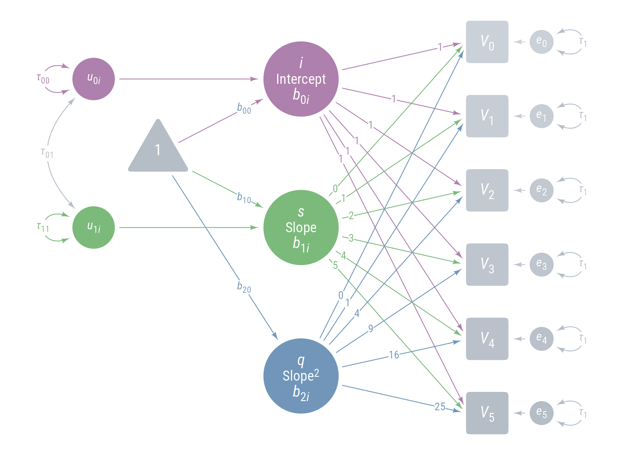
Model 4: Model 3 + Covariance between Random Intercepts and Slopes
Code
<- pd3 + ob_covariance (u_1i,color = cD,label = ob_label ("*τ*~01~" , color = cD))
Figure 20: Path Diagram for Model 4
<- " # Intercept i =~ 1 * voc_0 + 1 * voc_1 + 1 * voc_2 + 1 * voc_3 + 1 * voc_4 + 1 * voc_5 # Linear slope of time s =~ 0 * voc_0 + 1 * voc_1 + 2 * voc_2 + 3 * voc_3 + 4 * voc_4 + 5 * voc_5 # Acceleration effect of time (quadratic effect) q =~ 0 * voc_0 + 1 * voc_1 + 4 * voc_2 + 9 * voc_3 + 16 * voc_4 + 25 * voc_5 # Intercept, slope, and quadratic effects i ~ b_00 * 1 s ~ b_10 * 1 q ~ b_20 * 1 # Variances and covariances i ~~ tau_00 * i s ~~ tau_11 * s + tau_01 * i q ~~ 0 * q + 0 * s + 0 * i voc_0 ~~ e * voc_0 voc_1 ~~ e * voc_1 voc_2 ~~ e * voc_2 voc_3 ~~ e * voc_3 voc_4 ~~ e * voc_4 voc_5 ~~ e * voc_5 " <- growth (m_4, data = d_wide)parameters (fit_4, component = "all" )
# Loading

Link       | Coefficient |   SE |         95% CI |      p
---------------------------------------------------------
i =~ voc_0 |        1.00 | 0.00 | [ 1.00,  1.00] | < .001
i =~ voc_1 |        1.00 | 0.00 | [ 1.00,  1.00] | < .001
i =~ voc_2 |        1.00 | 0.00 | [ 1.00,  1.00] | < .001
i =~ voc_3 |        1.00 | 0.00 | [ 1.00,  1.00] | < .001
i =~ voc_4 |        1.00 | 0.00 | [ 1.00,  1.00] | < .001
i =~ voc_5 |        1.00 | 0.00 | [ 1.00,  1.00] | < .001
s =~ voc_0 |        0.00 | 0.00 | [ 0.00,  0.00] | < .001
s =~ voc_1 |        1.00 | 0.00 | [ 1.00,  1.00] | < .001
s =~ voc_2 |        2.00 | 0.00 | [ 2.00,  2.00] | < .001
s =~ voc_3 |        3.00 | 0.00 | [ 3.00,  3.00] | < .001
s =~ voc_4 |        4.00 | 0.00 | [ 4.00,  4.00] | < .001
s =~ voc_5 |        5.00 | 0.00 | [ 5.00,  5.00] | < .001
q =~ voc_0 |        0.00 | 0.00 | [ 0.00,  0.00] | < .001
q =~ voc_1 |        1.00 | 0.00 | [ 1.00,  1.00] | < .001
q =~ voc_2 |        4.00 | 0.00 | [ 4.00,  4.00] | < .001
q =~ voc_3 |        9.00 | 0.00 | [ 9.00,  9.00] | < .001
q =~ voc_4 |       16.00 | 0.00 | [16.00, 16.00] | < .001
q =~ voc_5 |       25.00 | 0.00 | [25.00, 25.00] | < .001

# Mean

Link         | Coefficient |   SE |         95% CI |      z |      p
--------------------------------------------------------------------
i ~1  (b_00) |       51.96 | 1.99 | [48.05, 55.86] |  26.08 | < .001
s ~1  (b_10) |       15.25 | 0.40 | [14.47, 16.03] |  38.49 | < .001
q ~1  (b_20) |       -1.01 | 0.03 | [-1.08, -0.94] | -29.14 | < .001
voc_0 ~1     |        0.00 | 0.00 | [ 0.00,  0.00] |        | < .001
voc_1 ~1     |        0.00 | 0.00 | [ 0.00,  0.00] |        | < .001
voc_2 ~1     |        0.00 | 0.00 | [ 0.00,  0.00] |        | < .001
voc_3 ~1     |        0.00 | 0.00 | [ 0.00,  0.00] |        | < .001
voc_4 ~1     |        0.00 | 0.00 | [ 0.00,  0.00] |        | < .001
voc_5 ~1     |        0.00 | 0.00 | [ 0.00,  0.00] |        | < .001

# Variance

Link               | Coefficient |    SE |           95% CI |     z |      p
----------------------------------------------------------------------------
i ~~ i (tau_00)    |      786.65 | 79.14 | [631.54, 941.75] |  9.94 | < .001
s ~~ s (tau_11)    |       24.86 |  2.54 | [ 19.89,  29.84] |  9.80 | < .001
q ~~ q             |        0.00 |  0.00 | [  0.00,   0.00] |       | < .001
voc_0 ~~ voc_0 (e) |        9.00 |  0.45 | [  8.12,   9.89] | 20.00 | < .001
voc_1 ~~ voc_1 (e) |        9.00 |  0.45 | [  8.12,   9.89] | 20.00 | < .001
voc_2 ~~ voc_2 (e) |        9.00 |  0.45 | [  8.12,   9.89] | 20.00 | < .001
voc_3 ~~ voc_3 (e) |        9.00 |  0.45 | [  8.12,   9.89] | 20.00 | < .001
voc_4 ~~ voc_4 (e) |        9.00 |  0.45 | [  8.12,   9.89] | 20.00 | < .001
voc_5 ~~ voc_5 (e) |        9.00 |  0.45 | [  8.12,   9.89] | 20.00 | < .001

# Correlation

Link            | Coefficient |    SE |          95% CI |    z |      p
-----------------------------------------------------------------------
i ~~ s (tau_01) |        3.71 | 10.02 | [-15.93, 23.36] | 0.37 | 0.711
s ~~ q          |        0.00 |  0.00 | [  0.00,  0.00] |      | < .001
i ~~ q          |        0.00 |  0.00 | [  0.00,  0.00] |      | < .001
# Compare new model with the previous models test_likelihoodratio (fit_0, fit_1, fit_2, fit_3, fit_4)
# Likelihood-Ratio-Test (LRT) for Model Comparison

Model |   Type | df | df_diff |    Chi2 |      p
------------------------------------------------
fit_0 | lavaan | 24 |       1 | 3228.27 | < .001
fit_1 | lavaan | 23 |       1 | 1722.61 | < .001
fit_2 | lavaan | 22 |       1 | 1646.01 | < .001
fit_3 | lavaan | 21 |       1 |   19.75 |  0.711
fit_4 | lavaan | 20 |         |   19.61 |
compare_performance (fit_0, fit_1, fit_2, fit_3, fit_4, metrics = my_metrics)
# Comparison of Model Performance Indices

Name  |  Model |   CFI |  NNFI |  AGFI | RMSEA
----------------------------------------------
fit_0 | lavaan | 0.121 | 0.450 | 0.426 | 0.817
fit_1 | lavaan | 0.534 | 0.696 | 0.726 | 0.608
fit_2 | lavaan | 0.554 | 0.696 | 0.709 | 0.608
fit_3 | lavaan | 1.000 | 1.000 | 0.992 | 0.000
fit_4 | lavaan | 1.000 | 1.000 | 0.992 | 0.000
The covariance is not significantly different from 0. I am going to leave it in for now because I want to test the random quadratic effect.
Code
ggplot (d, aes (time, vocabulary)) + :: geom_quasirandom (width = .2 , size = .5 , alpha = .5 ) + geom_line (data = predict (fit_4) %>% as_tibble () %>% mutate (across (everything (), .fns = as.numeric)) %>% mutate (person_id = dplyr:: row_number ()) %>% crossing (time = 0 : 5 ) %>% mutate (vocabulary = i + s * time + q * time^ 2 ),aes (group = person_id),alpha = .25 ,+ stat_function (data = tibble (x = 0 : 5 ),geom = "line" ,fun = \(x) coef (fit_4)["b_00" ] + coef (fit_4)["b_10" ] * x + coef (fit_4)["b_20" ] * (x^ 2 ),inherit.aes = F,color = "dodgerblue3" ,linewidth = 2 + theme_minimal (base_size = 20 , base_family = my_font) + labs (x = "Time" , y = "Vocabulary" )
Figure 21: Model 4: Predicted Vocabulary Over Time (Model 3 + Correlated Slopes and Intercepts)
lmer (vocabulary ~ 1 + time + I (time ^ 2 ) + (1 + time | person_id), data = d, REML = FALSE ) %>% tab_model ()
vocabulary
Predictors
Estimates
CI
p
(Intercept)
51.96
48.05 – 55.87
<0.001
time
15.25
14.47 – 16.03
<0.001
time^2
-1.01
-1.08 – -0.94
<0.001
Random Effects
σ2
9.00
τ00 person_id
786.64
τ11 person_id.time
24.86
ρ01 person_id
0.03
ICC
0.99
N person_id
200
Observations
1200
Marginal R2 / Conditional R2
0.229 / 0.993
Table 11: HLM Model Analogous to Model 4
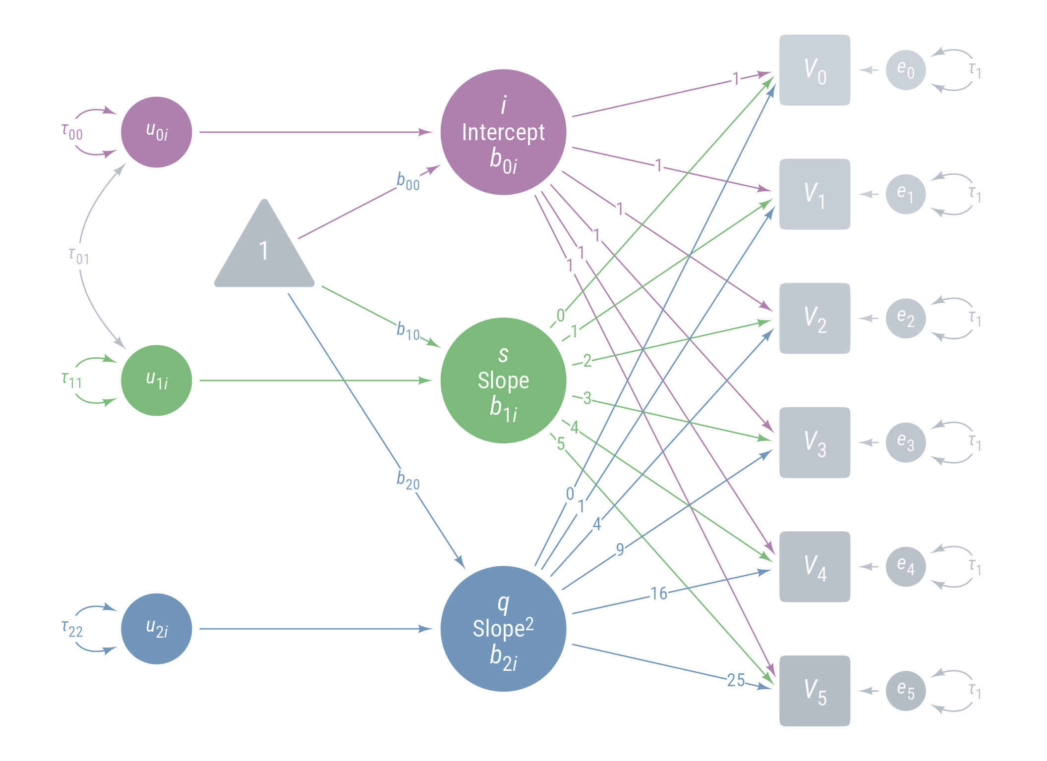
Model 5: Model 4 + Random Quadratic Effect
Code
<- pd4 + <- my_error (radius = 1 ,label = my_error_label ("*u*~2*i*~" ),fill = cC) %>% place (q, "left" , left)} + my_connect (u_2i, q, color = cC) + ob_variance (where = "west" ,color = cC,looseness = 1.75 ,label = ob_label (paste0 ("*τ*~22~" ), color = cC)
Figure 22: Path Diagram for Model 5
<- " # Intercept i =~ 1 * voc_0 + 1 * voc_1 + 1 * voc_2 + 1 * voc_3 + 1 * voc_4 + 1 * voc_5 # Linear slope of time s =~ 0 * voc_0 + 1 * voc_1 + 2 * voc_2 + 3 * voc_3 + 4 * voc_4 + 5 * voc_5 # Acceleration effect of time (quadratic effect) q =~ 0 * voc_0 + 1 * voc_1 + 4 * voc_2 + 9 * voc_3 + 16 * voc_4 + 25 * voc_5 # Intercept, slope, and quadratic effects i ~ b_00 * 1 s ~ b_10 * 1 q ~ b_20 * 1 # Variances and covariances i ~~ tau_00 * i s ~~ tau_11 * s + tau_01 * i q ~~ tau_22 * q + 0 * s + 0 * i voc_0 ~~ e * voc_0 voc_1 ~~ e * voc_1 voc_2 ~~ e * voc_2 voc_3 ~~ e * voc_3 voc_4 ~~ e * voc_4 voc_5 ~~ e * voc_5 " <- growth (m_5, data = d_wide)parameters (fit_5, component = "all" )
# Loading

Link       | Coefficient |   SE |         95% CI |      p
---------------------------------------------------------
i =~ voc_0 |        1.00 | 0.00 | [ 1.00,  1.00] | < .001
i =~ voc_1 |        1.00 | 0.00 | [ 1.00,  1.00] | < .001
i =~ voc_2 |        1.00 | 0.00 | [ 1.00,  1.00] | < .001
i =~ voc_3 |        1.00 | 0.00 | [ 1.00,  1.00] | < .001
i =~ voc_4 |        1.00 | 0.00 | [ 1.00,  1.00] | < .001
i =~ voc_5 |        1.00 | 0.00 | [ 1.00,  1.00] | < .001
s =~ voc_0 |        0.00 | 0.00 | [ 0.00,  0.00] | < .001
s =~ voc_1 |        1.00 | 0.00 | [ 1.00,  1.00] | < .001
s =~ voc_2 |        2.00 | 0.00 | [ 2.00,  2.00] | < .001
s =~ voc_3 |        3.00 | 0.00 | [ 3.00,  3.00] | < .001
s =~ voc_4 |        4.00 | 0.00 | [ 4.00,  4.00] | < .001
s =~ voc_5 |        5.00 | 0.00 | [ 5.00,  5.00] | < .001
q =~ voc_0 |        0.00 | 0.00 | [ 0.00,  0.00] | < .001
q =~ voc_1 |        1.00 | 0.00 | [ 1.00,  1.00] | < .001
q =~ voc_2 |        4.00 | 0.00 | [ 4.00,  4.00] | < .001
q =~ voc_3 |        9.00 | 0.00 | [ 9.00,  9.00] | < .001
q =~ voc_4 |       16.00 | 0.00 | [16.00, 16.00] | < .001
q =~ voc_5 |       25.00 | 0.00 | [25.00, 25.00] | < .001

# Mean

Link         | Coefficient |   SE |         95% CI |      z |      p
--------------------------------------------------------------------
i ~1  (b_00) |       51.96 | 1.99 | [48.06, 55.86] |  26.10 | < .001
s ~1  (b_10) |       15.25 | 0.39 | [14.49, 16.01] |  39.50 | < .001
q ~1  (b_20) |       -1.01 | 0.04 | [-1.09, -0.94] | -26.85 | < .001
voc_0 ~1     |        0.00 | 0.00 | [ 0.00,  0.00] |        | < .001
voc_1 ~1     |        0.00 | 0.00 | [ 0.00,  0.00] |        | < .001
voc_2 ~1     |        0.00 | 0.00 | [ 0.00,  0.00] |        | < .001
voc_3 ~1     |        0.00 | 0.00 | [ 0.00,  0.00] |        | < .001
voc_4 ~1     |        0.00 | 0.00 | [ 0.00,  0.00] |        | < .001
voc_5 ~1     |        0.00 | 0.00 | [ 0.00,  0.00] |        | < .001

# Variance

Link               | Coefficient |    SE |           95% CI |     z |      p
----------------------------------------------------------------------------
i ~~ i (tau_00)    |      785.74 | 79.07 | [630.77, 940.71] |  9.94 | < .001
s ~~ s (tau_11)    |       23.68 |  2.56 | [ 18.66,  28.71] |  9.24 | < .001
q ~~ q (tau_22)    |        0.06 |  0.03 | [  0.01,   0.11] |  2.25 | 0.024
voc_0 ~~ voc_0 (e) |        8.45 |  0.47 | [  7.53,   9.36] | 18.07 | < .001
voc_1 ~~ voc_1 (e) |        8.45 |  0.47 | [  7.53,   9.36] | 18.07 | < .001
voc_2 ~~ voc_2 (e) |        8.45 |  0.47 | [  7.53,   9.36] | 18.07 | < .001
voc_3 ~~ voc_3 (e) |        8.45 |  0.47 | [  7.53,   9.36] | 18.07 | < .001
voc_4 ~~ voc_4 (e) |        8.45 |  0.47 | [  7.53,   9.36] | 18.07 | < .001
voc_5 ~~ voc_5 (e) |        8.45 |  0.47 | [  7.53,   9.36] | 18.07 | < .001

# Correlation

Link            | Coefficient |    SE |          95% CI |    z |      p
-----------------------------------------------------------------------
i ~~ s (tau_01) |        4.94 | 10.01 | [-14.68, 24.56] | 0.49 | 0.622
s ~~ q          |        0.00 |  0.00 | [  0.00,  0.00] |      | < .001
i ~~ q          |        0.00 |  0.00 | [  0.00,  0.00] |      | < .001
# Compare new model with the previous models test_likelihoodratio (fit_0, fit_1, fit_2, fit_3, fit_4, fit_5)
# Likelihood-Ratio-Test (LRT) for Model Comparison

Model |   Type | df | df_diff |    Chi2 |      p
------------------------------------------------
fit_0 | lavaan | 24 |       1 | 3228.27 | < .001
fit_1 | lavaan | 23 |       1 | 1722.61 | < .001
fit_2 | lavaan | 22 |       1 | 1646.01 | < .001
fit_3 | lavaan | 21 |       1 |   19.75 |  0.711
fit_4 | lavaan | 20 |       1 |   19.61 |  0.012
fit_5 | lavaan | 19 |         |   13.23 |
compare_performance (fit_0, fit_1, fit_2, fit_3, fit_4, fit_5, metrics = c ())
# Comparison of Model Performance Indices

Name  |  Model |     Chi2 | Chi2_df | p (Chi2) | Baseline(15) | p (Baseline)
----------------------------------------------------------------------------
fit_0 | lavaan | 3228.267 |  24.000 |   < .001 |     3659.200 |       < .001
fit_1 | lavaan | 1722.613 |  23.000 |   < .001 |     3659.200 |       < .001
fit_2 | lavaan | 1646.015 |  22.000 |   < .001 |     3659.200 |       < .001
fit_3 | lavaan |   19.752 |  21.000 |   0.537  |     3659.200 |       < .001
fit_4 | lavaan |   19.615 |  20.000 |   0.482  |     3659.200 |       < .001
fit_5 | lavaan |   13.233 |  19.000 |   0.826  |     3659.200 |       < .001

Name  |   GFI |  AGFI | NFI |  NNFI |   CFI | RMSEA |      RMSEA  CI
--------------------------------------------------------------------
fit_0 | 0.489 | 0.426 |     | 0.450 | 0.121 | 0.817 | [0.793, 0.841]
fit_1 | 0.767 | 0.726 |     | 0.696 | 0.534 | 0.608 | [0.584, 0.632]
fit_2 | 0.763 | 0.709 |     | 0.696 | 0.554 | 0.608 | [0.583, 0.633]
fit_3 | 0.994 | 0.992 |     | 1.000 | 1.000 | 0.000 | [0.000, 0.056]
fit_4 | 0.994 | 0.992 |     | 1.000 | 1.000 | 0.000 | [0.000, 0.060]
fit_5 | 0.996 | 0.994 |     | 1.001 | 1.000 | 0.000 | [0.000, 0.038]

Name  | p (RMSEA) |     RMR |  SRMR | RFI |  PNFI |   IFI |   RNI
-----------------------------------------------------------------
fit_0 |    < .001 | 222.006 | 0.357 |     | 0.188 | 0.119 | 0.121
fit_1 |    < .001 | 160.723 | 0.154 |     | 0.811 | 0.533 | 0.534
fit_2 |    < .001 | 160.688 | 0.148 |     | 0.807 | 0.553 | 0.554
fit_3 |    0.916  |  19.138 | 0.017 |     | 1.392 | 1.000 | 1.000
fit_4 |    0.889  |   6.180 | 0.006 |     | 1.326 | 1.000 | 1.000
fit_5 |    0.982  |   7.453 | 0.007 |     | 1.262 | 1.002 | 1.002

Name  | Loglikelihood |   AIC (weights) |   BIC (weights) | BIC_adjusted
------------------------------------------------------------------------
fit_0 |     -5642.273 | 11290.5 (<.001) | 11300.4 (<.001) |    11290.938
fit_1 |     -4889.446 |  9786.9 (<.001) |  9800.1 (<.001) |     9787.413
fit_2 |     -4851.147 |  9712.3 (<.001) |  9728.8 (<.001) |     9712.945
fit_3 |     -4038.016 |  8088.0 (0.203) |  8107.8 (0.829) |     8088.813
fit_4 |     -4037.947 |  8089.9 (0.080) |  8113.0 (0.063) |     8090.806
fit_5 |     -4034.756 |  8085.5 (0.717) |  8111.9 (0.108) |     8086.554
Let’s keep the random quadratic effect.
Code
ggplot (d, aes (time, vocabulary)) + :: geom_quasirandom (width = .2 , size = .5 , alpha = .5 ) + geom_line (data = predict (fit_5) %>% as_tibble () %>% mutate (across (everything (), .fns = as.numeric)) %>% mutate (person_id = dplyr:: row_number ()) %>% crossing (time = 0 : 5 ) %>% mutate (vocabulary = i + s * time + q * time^ 2 ),aes (group = person_id),alpha = .25 ,+ stat_function (data = tibble (x = 0 : 5 ),geom = "line" ,fun = \(x) coef (fit_5)["b_00" ] + coef (fit_5)["b_10" ] * x + coef (fit_5)["b_20" ] * (x^ 2 ),inherit.aes = F,color = "dodgerblue3" ,linewidth = 2 + theme_minimal (base_size = 20 , base_family = my_font) + labs (x = "Time" , y = "Vocabulary" )
Figure 23: Model 5: Predicted Vocabulary Over Time (Model 4 + Random Quadratic Effect of Time)
lmer (vocabulary ~ 1 + time + I (time ^ 2 ) + 1 + time | person_id) + 0 + I (time ^ 2 ) | person_id), data = d, REML = FALSE ) %>% tab_model ()
vocabulary
Predictors
Estimates
CI
p
(Intercept)
51.96
48.05 – 55.86
<0.001
time
15.25
14.49 – 16.01
<0.001
time^2
-1.01
-1.09 – -0.94
<0.001
Random Effects
σ2
8.45
τ00 person_id
785.73
τ11 person_id.time
23.68
τ11 person_id.I(time^2)
0.06
ρ01 person_id
0.04
ICC
0.99
N person_id
200
Observations
1200
Marginal R2 / Conditional R2
0.230 / 0.994
Table 12: HLM Model Analogous to Model 5
Model 6: Model 5 + Correlations with Random Quadratic Effects
Code
<- pd5 + ob_covariance (bind (c (u_2i, u_2i)),bind (c (u_0i, u_1i)),color = cD,label = ob_label (paste0 ("*τ*~" , c (0 , 1 ), c (2 , 2 ), "~" ), color = cD))
Figure 24: Path Diagram for Model 6
Now lets allow the covariance between the quadratic effect and the linear and intercept to be non-zero:
<- " # Intercept i =~ 1 * voc_0 + 1 * voc_1 + 1 * voc_2 + 1 * voc_3 + 1 * voc_4 + 1 * voc_5 # Linear slope of time s =~ 0 * voc_0 + 1 * voc_1 + 2 * voc_2 + 3 * voc_3 + 4 * voc_4 + 5 * voc_5 # Acceleration effect of time (quadratic effect) q =~ 0 * voc_0 + 1 * voc_1 + 4 * voc_2 + 9 * voc_3 + 16 * voc_4 + 25 * voc_5 # Intercept, slope, and quadratic effects i ~ b_00 * 1 s ~ b_10 * 1 q ~ b_20 * 1 # Variances and covariances i ~~ tau_00 * i s ~~ tau_11 * s + tau_01 * i q ~~ tau_22 * q + tau_12 * s + tau_02 * i voc_0 ~~ e * voc_0 voc_1 ~~ e * voc_1 voc_2 ~~ e * voc_2 voc_3 ~~ e * voc_3 voc_4 ~~ e * voc_4 voc_5 ~~ e * voc_5 " <- growth (m_6, data = d_wide)parameters (fit_6, component = "all" )
# Loading

Link       | Coefficient |   SE |         95% CI |      p
---------------------------------------------------------
i =~ voc_0 |        1.00 | 0.00 | [ 1.00,  1.00] | < .001
i =~ voc_1 |        1.00 | 0.00 | [ 1.00,  1.00] | < .001
i =~ voc_2 |        1.00 | 0.00 | [ 1.00,  1.00] | < .001
i =~ voc_3 |        1.00 | 0.00 | [ 1.00,  1.00] | < .001
i =~ voc_4 |        1.00 | 0.00 | [ 1.00,  1.00] | < .001
i =~ voc_5 |        1.00 | 0.00 | [ 1.00,  1.00] | < .001
s =~ voc_0 |        0.00 | 0.00 | [ 0.00,  0.00] | < .001
s =~ voc_1 |        1.00 | 0.00 | [ 1.00,  1.00] | < .001
s =~ voc_2 |        2.00 | 0.00 | [ 2.00,  2.00] | < .001
s =~ voc_3 |        3.00 | 0.00 | [ 3.00,  3.00] | < .001
s =~ voc_4 |        4.00 | 0.00 | [ 4.00,  4.00] | < .001
s =~ voc_5 |        5.00 | 0.00 | [ 5.00,  5.00] | < .001
q =~ voc_0 |        0.00 | 0.00 | [ 0.00,  0.00] | < .001
q =~ voc_1 |        1.00 | 0.00 | [ 1.00,  1.00] | < .001
q =~ voc_2 |        4.00 | 0.00 | [ 4.00,  4.00] | < .001
q =~ voc_3 |        9.00 | 0.00 | [ 9.00,  9.00] | < .001
q =~ voc_4 |       16.00 | 0.00 | [16.00, 16.00] | < .001
q =~ voc_5 |       25.00 | 0.00 | [25.00, 25.00] | < .001

# Mean

Link         | Coefficient |   SE |         95% CI |      z |      p
--------------------------------------------------------------------
i ~1  (b_00) |       51.96 | 1.99 | [48.06, 55.85] |  26.13 | < .001
s ~1  (b_10) |       15.25 | 0.39 | [14.48, 16.02] |  38.78 | < .001
q ~1  (b_20) |       -1.01 | 0.04 | [-1.09, -0.94] | -26.39 | < .001
voc_0 ~1     |        0.00 | 0.00 | [ 0.00,  0.00] |        | < .001
voc_1 ~1     |        0.00 | 0.00 | [ 0.00,  0.00] |        | < .001
voc_2 ~1     |        0.00 | 0.00 | [ 0.00,  0.00] |        | < .001
voc_3 ~1     |        0.00 | 0.00 | [ 0.00,  0.00] |        | < .001
voc_4 ~1     |        0.00 | 0.00 | [ 0.00,  0.00] |        | < .001
voc_5 ~1     |        0.00 | 0.00 | [ 0.00,  0.00] |        | < .001

# Variance

Link               | Coefficient |    SE |           95% CI |     z |      p
----------------------------------------------------------------------------
i ~~ i (tau_00)    |      783.75 | 79.06 | [628.79, 938.70] |  9.91 | < .001
s ~~ s (tau_11)    |       24.86 |  3.11 | [ 18.76,  30.96] |  7.99 | < .001
q ~~ q (tau_22)    |        0.07 |  0.03 | [  0.01,   0.13] |  2.19 | 0.029
voc_0 ~~ voc_0 (e) |        8.35 |  0.48 | [  7.40,   9.29] | 17.32 | < .001
voc_1 ~~ voc_1 (e) |        8.35 |  0.48 | [  7.40,   9.29] | 17.32 | < .001
voc_2 ~~ voc_2 (e) |        8.35 |  0.48 | [  7.40,   9.29] | 17.32 | < .001
voc_3 ~~ voc_3 (e) |        8.35 |  0.48 | [  7.40,   9.29] | 17.32 | < .001
voc_4 ~~ voc_4 (e) |        8.35 |  0.48 | [  7.40,   9.29] | 17.32 | < .001
voc_5 ~~ voc_5 (e) |        8.35 |  0.48 | [  7.40,   9.29] | 17.32 | < .001

# Correlation

Link            | Coefficient |    SE |          95% CI |     z |     p
-----------------------------------------------------------------------
i ~~ s (tau_01) |        6.07 | 11.06 | [-15.61, 27.75] |  0.55 | 0.583
s ~~ q (tau_12) |       -0.17 |  0.24 | [ -0.64,  0.30] | -0.71 | 0.475
i ~~ q (tau_02) |       -0.37 |  1.08 | [ -2.48,  1.75] | -0.34 | 0.732
# Compare new model with the previous models test_likelihoodratio (fit_0, fit_1, fit_2, fit_3, fit_4, fit_5, fit_6)
# Likelihood-Ratio-Test (LRT) for Model Comparison

Model |   Type | df | df_diff |    Chi2 |      p
------------------------------------------------
fit_0 | lavaan | 24 |       1 | 3228.27 | < .001
fit_1 | lavaan | 23 |       1 | 1722.61 | < .001
fit_2 | lavaan | 22 |       1 | 1646.01 | < .001
fit_3 | lavaan | 21 |       1 |   19.75 |  0.711
fit_4 | lavaan | 20 |       1 |   19.61 |  0.012
fit_5 | lavaan | 19 |       2 |   13.23 |  0.714
fit_6 | lavaan | 17 |         |   12.56 |
compare_performance (fit_0, fit_1, fit_2, fit_3, fit_4, fit_5, fit_6, metrics = my_metrics)
# Comparison of Model Performance Indices

Name  |  Model |   CFI |  NNFI |  AGFI | RMSEA
----------------------------------------------
fit_0 | lavaan | 0.121 | 0.450 | 0.426 | 0.817
fit_1 | lavaan | 0.534 | 0.696 | 0.726 | 0.608
fit_2 | lavaan | 0.554 | 0.696 | 0.709 | 0.608
fit_3 | lavaan | 1.000 | 1.000 | 0.992 | 0.000
fit_4 | lavaan | 1.000 | 1.000 | 0.992 | 0.000
fit_5 | lavaan | 1.000 | 1.001 | 0.994 | 0.000
fit_6 | lavaan | 1.000 | 1.001 | 0.993 | 0.000
These effects are not needed. We have the option of trimming them now, but I am going to wait a little longer.
Code
ggplot (d, aes (time, vocabulary)) + :: geom_quasirandom (width = .2 , size = .5 , alpha = .5 ) + geom_line (data = predict (fit_6) %>% as_tibble () %>% mutate (across (everything (), .fns = as.numeric)) %>% mutate (person_id = dplyr:: row_number ()) %>% crossing (time = 0 : 5 ) %>% mutate (vocabulary = i + s * time + q * time^ 2 ),aes (group = person_id),alpha = .25 ,+ stat_function (data = tibble (x = 0 : 5 ),geom = "line" ,fun = \(x) coef (fit_6)["b_00" ] + coef (fit_6)["b_10" ] * x + coef (fit_6)["b_20" ] * (x^ 2 ),inherit.aes = F,color = "dodgerblue3" ,linewidth = 2 + theme_minimal (base_size = 20 , base_family = my_font) + labs (x = "Time" , y = "Vocabulary" )
Figure 25: Model 6: Predicted Vocabulary Over Time (Model 5 + All Random Effects Correlated)
lmer (vocabulary ~ 1 + time + I (time ^ 2 ) + 1 + time + I (time ^ 2 ) | person_id), data = d, REML = FALSE ) %>% tab_model ()
vocabulary
Predictors
Estimates
CI
p
(Intercept)
51.96
48.06 – 55.86
<0.001
time
15.25
14.48 – 16.02
<0.001
time^2
-1.01
-1.09 – -0.94
<0.001
Random Effects
σ2
8.35
τ00 person_id
783.68
τ11 person_id.time
24.87
τ11 person_id.I(time^2)
0.07
ρ01
0.04
-0.05
ICC
0.99
N person_id
200
Observations
1200
Marginal R2 / Conditional R2
0.229 / 0.994
Table 13: HLM Model Analogous to Model 6
Model 7: Model 6 + Treatment Effects
Code
<- pd6 + <- my_observed (intersection (connect (u_2i, s), connect (u_1i, q)) + ob_point (- 1.85 , 0 ),a = 1.75 ,b = 1.75 ,fill = cD,label = my_observed_label ("Intervention" , size = 15 )+ <- my_connect (intervention, bind (c (i, s, q)), color = my_colors)} + ob_label (paste0 ("*b*~" , 0 : 2 , "1~" ),intersection (lt1, vl),label.padding = margin (2 ),color = my_colors
Figure 26: Path Diagram for Model 7
I am going to add all three treatment effects at the same time. We could do them one-at-a-time, but no important theoretical question would be answered by doing so. I am mostly interested in the interactions of treatment and the time variables.
<- " # Intercept i =~ 1 * voc_0 + 1 * voc_1 + 1 * voc_2 + 1 * voc_3 + 1 * voc_4 + 1 * voc_5 # Linear slope of time s =~ 0 * voc_0 + 1 * voc_1 + 2 * voc_2 + 3 * voc_3 + 4 * voc_4 + 5 * voc_5 # Acceleration effect of time (quadratic effect) q =~ 0 * voc_0 + 1 * voc_1 + 4 * voc_2 + 9 * voc_3 + 16 * voc_4 + 25 * voc_5 # Intercept, slope, and quadratic effects i ~ b_00 * 1 + b_01 * intervention s ~ b_10 * 1 + b_11 * intervention q ~ b_20 * 1 + b_21 * intervention # Variances and covariances i ~~ tau_00 * i s ~~ tau_11 * s + tau_01 * i q ~~ tau_22 * q + tau_12 * s + tau_02 * i voc_0 ~~ e * voc_0 voc_1 ~~ e * voc_1 voc_2 ~~ e * voc_2 voc_3 ~~ e * voc_3 voc_4 ~~ e * voc_4 voc_5 ~~ e * voc_5 " <- growth (m_7, data = d_wide)parameters (fit_7, component = "all" )
# Loading

Link       | Coefficient |   SE |         95% CI |      p
---------------------------------------------------------
i =~ voc_0 |        1.00 | 0.00 | [ 1.00,  1.00] | < .001
i =~ voc_1 |        1.00 | 0.00 | [ 1.00,  1.00] | < .001
i =~ voc_2 |        1.00 | 0.00 | [ 1.00,  1.00] | < .001
i =~ voc_3 |        1.00 | 0.00 | [ 1.00,  1.00] | < .001
i =~ voc_4 |        1.00 | 0.00 | [ 1.00,  1.00] | < .001
i =~ voc_5 |        1.00 | 0.00 | [ 1.00,  1.00] | < .001
s =~ voc_0 |        0.00 | 0.00 | [ 0.00,  0.00] | < .001
s =~ voc_1 |        1.00 | 0.00 | [ 1.00,  1.00] | < .001
s =~ voc_2 |        2.00 | 0.00 | [ 2.00,  2.00] | < .001
s =~ voc_3 |        3.00 | 0.00 | [ 3.00,  3.00] | < .001
s =~ voc_4 |        4.00 | 0.00 | [ 4.00,  4.00] | < .001
s =~ voc_5 |        5.00 | 0.00 | [ 5.00,  5.00] | < .001
q =~ voc_0 |        0.00 | 0.00 | [ 0.00,  0.00] | < .001
q =~ voc_1 |        1.00 | 0.00 | [ 1.00,  1.00] | < .001
q =~ voc_2 |        4.00 | 0.00 | [ 4.00,  4.00] | < .001
q =~ voc_3 |        9.00 | 0.00 | [ 9.00,  9.00] | < .001
q =~ voc_4 |       16.00 | 0.00 | [16.00, 16.00] | < .001
q =~ voc_5 |       25.00 | 0.00 | [25.00, 25.00] | < .001

# Mean

Link            | Coefficient |   SE |         95% CI |      z |      p
-----------------------------------------------------------------------
i ~1  (b_00)    |       52.00 | 2.87 | [46.38, 57.63] |  18.12 | < .001
s ~1  (b_10)    |       10.50 | 0.32 | [ 9.86, 11.14] |  32.39 | < .001
q ~1  (b_20)    |       -1.06 | 0.06 | [-1.16, -0.95] | -19.15 | < .001
voc_0 ~1        |        0.00 | 0.00 | [ 0.00,  0.00] |        | < .001
voc_1 ~1        |        0.00 | 0.00 | [ 0.00,  0.00] |        | < .001
voc_2 ~1        |        0.00 | 0.00 | [ 0.00,  0.00] |        | < .001
voc_3 ~1        |        0.00 | 0.00 | [ 0.00,  0.00] |        | < .001
voc_4 ~1        |        0.00 | 0.00 | [ 0.00,  0.00] |        | < .001
voc_5 ~1        |        0.00 | 0.00 | [ 0.00,  0.00] |        | < .001
intervention ~1 |        0.52 | 0.00 | [ 0.52,  0.52] |        | < .001

# Regression

Link                    | Coefficient |   SE |         95% CI |     z |      p
------------------------------------------------------------------------------
i ~ intervention (b_01) |       -0.09 | 3.98 | [-7.89,  7.71] | -0.02 | 0.983
s ~ intervention (b_11) |        9.14 | 0.45 | [ 8.26, 10.02] | 20.33 | < .001
q ~ intervention (b_21) |        0.09 | 0.08 | [-0.06,  0.24] |  1.12 | 0.262

# Variance

Link                         | Coefficient |    SE |           95% CI |     z |      p
--------------------------------------------------------------------------------------
i ~~ i (tau_00)              |      783.74 | 79.06 | [628.79, 938.70] |  9.91 | < .001
s ~~ s (tau_11)              |        4.02 |  1.07 | [  1.93,   6.11] |  3.77 | < .001
q ~~ q (tau_22)              |        0.07 |  0.03 | [  0.01,   0.13] |  2.14 | 0.032
voc_0 ~~ voc_0 (e)           |        8.35 |  0.48 | [  7.40,   9.29] | 17.32 | < .001
voc_1 ~~ voc_1 (e)           |        8.35 |  0.48 | [  7.40,   9.29] | 17.32 | < .001
voc_2 ~~ voc_2 (e)           |        8.35 |  0.48 | [  7.40,   9.29] | 17.32 | < .001
voc_3 ~~ voc_3 (e)           |        8.35 |  0.48 | [  7.40,   9.29] | 17.32 | < .001
voc_4 ~~ voc_4 (e)           |        8.35 |  0.48 | [  7.40,   9.29] | 17.32 | < .001
voc_5 ~~ voc_5 (e)           |        8.35 |  0.48 | [  7.40,   9.29] | 17.32 | < .001
intervention ~~ intervention |        0.25 |  0.00 | [  0.25,   0.25] |       | < .001

# Correlation

Link            | Coefficient |   SE |         95% CI |     z |     p
---------------------------------------------------------------------
i ~~ s (tau_01) |        6.26 | 6.32 | [-6.13, 18.65] |  0.99 | 0.322
s ~~ q (tau_12) |       -0.37 | 0.17 | [-0.71, -0.03] | -2.12 | 0.034
i ~~ q (tau_02) |       -0.37 | 1.08 | [-2.48,  1.74] | -0.34 | 0.733
# Compare new model with the previous models test_likelihoodratio (fit_6, fit_7)
# Likelihood-Ratio-Test (LRT) for Model Comparison

Model |   Type | df | df_diff |  Chi2 |     p
---------------------------------------------
fit_6 | lavaan | 17 |         | 12.56 |
fit_7 | lavaan | 20 |       3 | 14.44 | 0.598
compare_performance (fit_6, fit_7, metrics = my_metrics)
# Comparison of Model Performance Indices

Name  |  Model |   CFI |  NNFI |  AGFI | RMSEA
----------------------------------------------
fit_6 | lavaan | 1.000 | 1.001 | 0.993 | 0.000
fit_7 | lavaan | 1.000 | 1.001 | 0.999 | 0.000
So the intervention effects improve the model fit. Specifically, the intervention predicts the slope such that the slope is steeper for the treatment group.
Code
<- lavPredictY (ynames = d_wide %>% select (starts_with ("voc_" )) %>% colnames (),xnames = "intervention" ,newdata = tibble (intervention = c (0 , 1 ),voc_0 = 0 ,voc_1 = 0 ,voc_2 = 0 ,voc_3 = 0 ,voc_4 = 0 ,voc_5 = 0 %>% as_tibble () %>% mutate (intervention = factor (c (0 , 1 ), labels = c ("Control" , "Treatment" ))) %>% pivot_longer (starts_with ("voc_" ),names_to = "time" ,names_prefix = "voc_" ,names_transform = list (time = as.integer),values_to = "vocabulary" ggplot (data = d %>% mutate (intervention = factor (labels = c ("Control" , "Treatment" ))), aes (time, vocabulary)) + :: geom_quasirandom (aes (color = intervention, group = intervention),width = .05 ,data = . %>% mutate (time = time + (as.numeric (intervention) - 1.5 ) / 6 ),size = .5 ,alpha = .5 + geom_line (data = my_predictions (fit_7) %>% mutate (intervention = factor (labels = c ("Control" , "Treatment" )aes (group = person_id, color = intervention),alpha = .3 ,linewidth = .5 + geom_line (data = pred_7,aes (group = intervention, color = intervention),linewidth = 3 + :: geom_labelline (data = pred_7,aes (color = intervention,group = intervention,label = interventionvjust = - .3 ,size = 6 ,family = my_font,fill = "#FFFFFFBB" ,text_only = T,linewidth = 0 ,label.padding = margin (1 , 1 , 1 , 1 ),hjust = .95 + theme_minimal (base_size = 20 , base_family = my_font) + theme (legend.position = "none" ) + scale_color_manual (values = c (Control = "dodgerblue4" ,Treatment = "forestgreen" + labs (x = "Time" , y = "Vocabulary" )
Figure 27: Model 7: Predicted Vocabulary by Intervention Group Over Time (Model 6 + Effects of Intervention on Intercept, Linear Effect of Time, and Quadratic Effect of Time)
lmer (vocabulary ~ 1 + time* intervention + I (time ^ 2 ) * intervention + 1 + time + I (time ^ 2 ) | person_id), data = d, REML = FALSE ) %>% tab_model ()
vocabulary
Predictors
Estimates
CI
p
(Intercept)
52.00
46.37 – 57.63
<0.001
time
10.50
9.86 – 11.14
<0.001
intervention
-0.09
-7.89 – 7.72
0.983
time^2
-1.06
-1.16 – -0.95
<0.001
time × intervention
9.14
8.26 – 10.02
<0.001
intervention × time^2
0.09
-0.06 – 0.24
0.262
Random Effects
σ2
8.35
τ00 person_id
783.75
τ11 person_id.time
4.02
τ11 person_id.I(time^2)
0.07
ρ01
0.11
-0.05
ICC
0.99
N person_id
200
Observations
1200
Marginal R2 / Conditional R2
0.381 / 0.994
Table 14: HLM Model Analogous to Model 7
Model 8: Model 7 + Autoregression Effect
Code
<- pd7 + my_connect (1 : 5 ],2 : 6 ],color = v@ fill[- 6 ],label = ob_label ("*r*" ,angle = 0 ,position = .4 ,size = 14 ,label.padding = margin ()resect = 1
Figure 28: Path Diagram for Model 8
Suppose that we want to add an autoregression effect to our latent growth model.
An autoregression allows for the residuals of earlier observed variables to have lasting effects on subsequent variables.
<- " # Intercept i =~ 1 * voc_0 + 1 * voc_1 + 1 * voc_2 + 1 * voc_3 + 1 * voc_4 + 1 * voc_5 # Linear slope of time s =~ 0 * voc_0 + 1 * voc_1 + 2 * voc_2 + 3 * voc_3 + 4 * voc_4 + 5 * voc_5 # Acceleration effect of time (quadratic effect) q =~ 0 * voc_0 + 1 * voc_1 + 4 * voc_2 + 9 * voc_3 + 16 * voc_4 + 25 * voc_5 # Intercept, slope, and quadratic effects i ~ b_00 * 1 + b_01 * intervention s ~ b_10 * 1 + b_11 * intervention q ~ b_20 * 1 + b_21 * intervention # Variances and covariances i ~~ tau_00 * i s ~~ tau_11 * s + tau_01 * i q ~~ tau_22 * q + tau_12 * s + tau_02 * i voc_0 ~~ e * voc_0 voc_1 ~~ e * voc_1 voc_2 ~~ e * voc_2 voc_3 ~~ e * voc_3 voc_4 ~~ e * voc_4 voc_5 ~~ e * voc_5 # Autoregression voc_1 ~ r * voc_0 voc_2 ~ r * voc_1 voc_3 ~ r * voc_2 voc_4 ~ r * voc_3 voc_5 ~ r * voc_4 " <- growth (m_8, data = d_wide)parameters (fit_8, component = "all" )
# Loading

Link       | Coefficient |   SE |         95% CI |      p
---------------------------------------------------------
i =~ voc_0 |        1.00 | 0.00 | [ 1.00,  1.00] | < .001
i =~ voc_1 |        1.00 | 0.00 | [ 1.00,  1.00] | < .001
i =~ voc_2 |        1.00 | 0.00 | [ 1.00,  1.00] | < .001
i =~ voc_3 |        1.00 | 0.00 | [ 1.00,  1.00] | < .001
i =~ voc_4 |        1.00 | 0.00 | [ 1.00,  1.00] | < .001
i =~ voc_5 |        1.00 | 0.00 | [ 1.00,  1.00] | < .001
s =~ voc_0 |        0.00 | 0.00 | [ 0.00,  0.00] | < .001
s =~ voc_1 |        1.00 | 0.00 | [ 1.00,  1.00] | < .001
s =~ voc_2 |        2.00 | 0.00 | [ 2.00,  2.00] | < .001
s =~ voc_3 |        3.00 | 0.00 | [ 3.00,  3.00] | < .001
s =~ voc_4 |        4.00 | 0.00 | [ 4.00,  4.00] | < .001
s =~ voc_5 |        5.00 | 0.00 | [ 5.00,  5.00] | < .001
q =~ voc_0 |        0.00 | 0.00 | [ 0.00,  0.00] | < .001
q =~ voc_1 |        1.00 | 0.00 | [ 1.00,  1.00] | < .001
q =~ voc_2 |        4.00 | 0.00 | [ 4.00,  4.00] | < .001
q =~ voc_3 |        9.00 | 0.00 | [ 9.00,  9.00] | < .001
q =~ voc_4 |       16.00 | 0.00 | [16.00, 16.00] | < .001
q =~ voc_5 |       25.00 | 0.00 | [25.00, 25.00] | < .001

# Mean

Link            | Coefficient |   SE |         95% CI |      z |      p
-----------------------------------------------------------------------
i ~1  (b_00)    |       52.01 | 2.87 | [46.38, 57.64] |  18.11 | < .001
s ~1  (b_10)    |       10.54 | 0.50 | [ 9.56, 11.52] |  21.03 | < .001
q ~1  (b_20)    |       -1.06 | 0.07 | [-1.21, -0.92] | -14.39 | < .001
voc_0 ~1        |        0.00 | 0.00 | [ 0.00,  0.00] |        | < .001
voc_1 ~1        |        0.00 | 0.00 | [ 0.00,  0.00] |        | < .001
voc_2 ~1        |        0.00 | 0.00 | [ 0.00,  0.00] |        | < .001
voc_3 ~1        |        0.00 | 0.00 | [ 0.00,  0.00] |        | < .001
voc_4 ~1        |        0.00 | 0.00 | [ 0.00,  0.00] |        | < .001
voc_5 ~1        |        0.00 | 0.00 | [ 0.00,  0.00] |        | < .001
intervention ~1 |        0.52 | 0.00 | [ 0.52,  0.52] |        | < .001

# Regression

Link                    | Coefficient |   SE |         95% CI |     z |      p
------------------------------------------------------------------------------
i ~ intervention (b_01) |       -0.09 | 3.98 | [-7.89,  7.71] | -0.02 | 0.982
s ~ intervention (b_11) |        9.14 | 0.45 | [ 8.26, 10.03] | 20.25 | < .001
q ~ intervention (b_21) |        0.09 | 0.08 | [-0.06,  0.24] |  1.13 | 0.261
voc_1 ~ voc_0 (r)       |   -1.06e-03 | 0.01 | [-0.02,  0.02] | -0.10 | 0.920
voc_2 ~ voc_1 (r)       |   -1.06e-03 | 0.01 | [-0.02,  0.02] | -0.10 | 0.920
voc_3 ~ voc_2 (r)       |   -1.06e-03 | 0.01 | [-0.02,  0.02] | -0.10 | 0.920
voc_4 ~ voc_3 (r)       |   -1.06e-03 | 0.01 | [-0.02,  0.02] | -0.10 | 0.920
voc_5 ~ voc_4 (r)       |   -1.06e-03 | 0.01 | [-0.02,  0.02] | -0.10 | 0.920

# Variance

Link                         | Coefficient |    SE |           95% CI |     z |      p
--------------------------------------------------------------------------------------
i ~~ i (tau_00)              |      784.05 | 79.15 | [628.92, 939.18] |  9.91 | < .001
s ~~ s (tau_11)              |        4.04 |  1.09 | [  1.91,   6.18] |  3.71 | < .001
q ~~ q (tau_22)              |        0.07 |  0.03 | [  0.01,   0.13] |  2.14 | 0.033
voc_0 ~~ voc_0 (e)           |        8.34 |  0.49 | [  7.38,   9.30] | 17.04 | < .001
voc_1 ~~ voc_1 (e)           |        8.34 |  0.49 | [  7.38,   9.30] | 17.04 | < .001
voc_2 ~~ voc_2 (e)           |        8.34 |  0.49 | [  7.38,   9.30] | 17.04 | < .001
voc_3 ~~ voc_3 (e)           |        8.34 |  0.49 | [  7.38,   9.30] | 17.04 | < .001
voc_4 ~~ voc_4 (e)           |        8.34 |  0.49 | [  7.38,   9.30] | 17.04 | < .001
voc_5 ~~ voc_5 (e)           |        8.34 |  0.49 | [  7.38,   9.30] | 17.04 | < .001
intervention ~~ intervention |        0.25 |  0.00 | [  0.25,   0.25] |       | < .001

# Correlation

Link            | Coefficient |   SE |         95% CI |     z |     p
---------------------------------------------------------------------
i ~~ s (tau_01) |        6.74 | 7.95 | [-8.84, 22.33] |  0.85 | 0.396
s ~~ q (tau_12) |       -0.37 | 0.18 | [-0.71, -0.03] | -2.11 | 0.034
i ~~ q (tau_02) |       -0.44 | 1.30 | [-2.98,  2.10] | -0.34 | 0.735
# Compare models test_likelihoodratio (fit_7, fit_8)
# Likelihood-Ratio-Test (LRT) for Model Comparison

Model |   Type | df | df_diff |  Chi2 |     p
---------------------------------------------
fit_7 | lavaan | 20 |       1 | 14.44 | 0.920
fit_8 | lavaan | 19 |         | 14.43 |
The autoregression parameter was not statistically significant. Comparing the two models revealed no difference in model fit. Thus, there appears to be no need of the autoregression parameter, once we have accounted for the latent growth.
Exercise
After a series of painful incidents in which several middle-schoolers were severely harassed and bullied by peers, the school principal decided to implement a school-wide social-emotional learning intervention that aims to give students verbal self-defense skills, encourage bystanders to become “upstanders” that defend bullied peers, and to create an overall sense of solidarity and belonging at the school. Each student’s sense of school belonging was measured before the intervention and for each of the 8 weeks of the intervention. Your task is to how school belonging increases in general and specifically for students who self-identify as having been bullied.
The data can be imported like so:
<- read_csv ("https://github.com/wjschne/EDUC8825/raw/main/belonging.csv" ,show_col_types = F
The data should look like this:
# A tibble: 6 × 11
     id bullied  sb_0  sb_1  sb_2  sb_3  sb_4  sb_5  sb_6  sb_7  sb_8
  <dbl> <chr>   <dbl> <dbl> <dbl> <dbl> <dbl> <dbl> <dbl> <dbl> <dbl>
1     1 No       83.7 111.   87.7  81.2 115.   105.  124.  142.  126.
2     2 No      106.   98.7  97.3 105.  109.   124.  127.  139.  147.
3     3 No       92.3  71.2  90.2  98.4  99.7  108.  109.  162.  152.
4     4 No       90.0  92.7  93.8  97.4  88.8  117.  122.  115.  142.
5     5 No      117.  106.  138.  138.  144.   167.  172.  168.  168.
6     6 No      128.  132.  123.  170.  162.   139.  160.  165.  143.
First let’s plot the data to see what we are looking at in Figure 29 .
%>% pivot_longer (- c (id, bullied),names_prefix = "sb_" ,names_to = "time" ,values_to = "belonging" %>% mutate (time = as.numeric (time)) %>% ggplot (aes (time, belonging)) + geom_line (aes (group = id, color = bullied), alpha = .3 ) + :: geom_smooth (aes (color = bullied),linewidth = 2 ,method = "lm" ,formula = "y ~ poly(x,2)"
Figure 29: Trajectory of change in self-rated sense of school belonging for bullied and non-bullied student during 8 weeks of an anti-bullying intervention.
It looks like both groups felt increasing levels of belonging, but that their trajectories of change differed. Let’s test this idea formally.
Using latent growth models, conduct the following tests:
Create a plain random intercept model. Call the intercept latent variable i, its intercept parameter b_00, and its variance tau_00. Set the observed variable’s variances equal using the parameter name tau_1.
<- " # Intercept i =~ 1 * sb_0 + 1 * sb_1 + 1 * sb_2 + 1 * sb_3 + 1 * sb_4 + 1 * sb_5 + 1 * sb_6 + 1 * sb_7 + 1 * sb_8 # Regression effects on latent variables i ~ b_00 * 1 # Variances and covariances i ~~ tau_00 * i sb_0 ~~ tau_1 * sb_0 sb_1 ~~ tau_1 * sb_1 sb_2 ~~ tau_1 * sb_2 sb_3 ~~ tau_1 * sb_3 sb_4 ~~ tau_1 * sb_4 sb_5 ~~ tau_1 * sb_5 sb_6 ~~ tau_1 * sb_6 sb_7 ~~ tau_1 * sb_7 sb_8 ~~ tau_1 * sb_8 " <- growth (m_0, data = d_belong)parameters (fit_0, component = "all" )
# Loading

Link      | Coefficient |   SE |       95% CI |      p
------------------------------------------------------
i =~ sb_0 |        1.00 | 0.00 | [1.00, 1.00] | < .001
i =~ sb_1 |        1.00 | 0.00 | [1.00, 1.00] | < .001
i =~ sb_2 |        1.00 | 0.00 | [1.00, 1.00] | < .001
i =~ sb_3 |        1.00 | 0.00 | [1.00, 1.00] | < .001
i =~ sb_4 |        1.00 | 0.00 | [1.00, 1.00] | < .001
i =~ sb_5 |        1.00 | 0.00 | [1.00, 1.00] | < .001
i =~ sb_6 |        1.00 | 0.00 | [1.00, 1.00] | < .001
i =~ sb_7 |        1.00 | 0.00 | [1.00, 1.00] | < .001
i =~ sb_8 |        1.00 | 0.00 | [1.00, 1.00] | < .001

# Mean

Link         | Coefficient |   SE |           95% CI |      z |      p
----------------------------------------------------------------------
i ~1  (b_00) |      129.94 | 1.05 | [127.88, 132.00] | 123.87 | < .001
sb_0 ~1      |        0.00 | 0.00 | [  0.00,   0.00] |        | < .001
sb_1 ~1      |        0.00 | 0.00 | [  0.00,   0.00] |        | < .001
sb_2 ~1      |        0.00 | 0.00 | [  0.00,   0.00] |        | < .001
sb_3 ~1      |        0.00 | 0.00 | [  0.00,   0.00] |        | < .001
sb_4 ~1      |        0.00 | 0.00 | [  0.00,   0.00] |        | < .001
sb_5 ~1      |        0.00 | 0.00 | [  0.00,   0.00] |        | < .001
sb_6 ~1      |        0.00 | 0.00 | [  0.00,   0.00] |        | < .001
sb_7 ~1      |        0.00 | 0.00 | [  0.00,   0.00] |        | < .001
sb_8 ~1      |        0.00 | 0.00 | [  0.00,   0.00] |        | < .001

# Variance

Link                 | Coefficient |    SE |           95% CI |     z |      p
------------------------------------------------------------------------------
i ~~ i (tau_00)      |      496.94 | 34.82 | [428.69, 565.18] | 14.27 | < .001
sb_0 ~~ sb_0 (tau_1) |      479.53 | 10.72 | [458.52, 500.55] | 44.72 | < .001
sb_1 ~~ sb_1 (tau_1) |      479.53 | 10.72 | [458.52, 500.55] | 44.72 | < .001
sb_2 ~~ sb_2 (tau_1) |      479.53 | 10.72 | [458.52, 500.55] | 44.72 | < .001
sb_3 ~~ sb_3 (tau_1) |      479.53 | 10.72 | [458.52, 500.55] | 44.72 | < .001
sb_4 ~~ sb_4 (tau_1) |      479.53 | 10.72 | [458.52, 500.55] | 44.72 | < .001
sb_5 ~~ sb_5 (tau_1) |      479.53 | 10.72 | [458.52, 500.55] | 44.72 | < .001
sb_6 ~~ sb_6 (tau_1) |      479.53 | 10.72 | [458.52, 500.55] | 44.72 | < .001
sb_7 ~~ sb_7 (tau_1) |      479.53 | 10.72 | [458.52, 500.55] | 44.72 | < .001
sb_8 ~~ sb_8 (tau_1) |      479.53 | 10.72 | [458.52, 500.55] | 44.72 | < .001
<- c ("CFI" , "NNFI" , "AGFI" , "RMSEA" , "AIC" , "BIC" )performance (fit_0, metrics = my_metrics)
# Indices of model performance

CFI   |  NNFI |  AGFI | RMSEA |       AIC |       BIC
-----------------------------------------------------
0.022 | 0.310 | 0.769 | 0.482 | 41721.454 | 41734.098
Evaluate whether adding a fixed linear effect of time is significant. Call the slope latent variable s, its intercept parameter b_10. Set s’s variance to 0, as well as its covariance with i.
<- " # Intercept i =~ 1 * sb_0 + 1 * sb_1 + 1 * sb_2 + 1 * sb_3 + 1 * sb_4 + 1 * sb_5 + 1 * sb_6 + 1 * sb_7 + 1 * sb_8 # Linear slope of time s =~ 0 * sb_0 + 1 * sb_1 + 2 * sb_2 + 3 * sb_3 + 4 * sb_4 + 5 * sb_5 + 6 * sb_6 + 7 * sb_7 + 8 * sb_8 # Regression effects on latent variables i ~ b_00 * 1 s ~ b_10 * 1 # Variances and covariances i ~~ tau_00 * i s ~~ 0 * s + 0 * i sb_0 ~~ tau_1 * sb_0 sb_1 ~~ tau_1 * sb_1 sb_2 ~~ tau_1 * sb_2 sb_3 ~~ tau_1 * sb_3 sb_4 ~~ tau_1 * sb_4 sb_5 ~~ tau_1 * sb_5 sb_6 ~~ tau_1 * sb_6 sb_7 ~~ tau_1 * sb_7 sb_8 ~~ tau_1 * sb_8 " <- growth (m_1, data = d_belong)parameters (fit_1, component = "all" )
# Loading

Link      | Coefficient |   SE |       95% CI |      p
------------------------------------------------------
i =~ sb_0 |        1.00 | 0.00 | [1.00, 1.00] | < .001
i =~ sb_1 |        1.00 | 0.00 | [1.00, 1.00] | < .001
i =~ sb_2 |        1.00 | 0.00 | [1.00, 1.00] | < .001
i =~ sb_3 |        1.00 | 0.00 | [1.00, 1.00] | < .001
i =~ sb_4 |        1.00 | 0.00 | [1.00, 1.00] | < .001
i =~ sb_5 |        1.00 | 0.00 | [1.00, 1.00] | < .001
i =~ sb_6 |        1.00 | 0.00 | [1.00, 1.00] | < .001
i =~ sb_7 |        1.00 | 0.00 | [1.00, 1.00] | < .001
i =~ sb_8 |        1.00 | 0.00 | [1.00, 1.00] | < .001
s =~ sb_0 |        0.00 | 0.00 | [0.00, 0.00] | < .001
s =~ sb_1 |        1.00 | 0.00 | [1.00, 1.00] | < .001
s =~ sb_2 |        2.00 | 0.00 | [2.00, 2.00] | < .001
s =~ sb_3 |        3.00 | 0.00 | [3.00, 3.00] | < .001
s =~ sb_4 |        4.00 | 0.00 | [4.00, 4.00] | < .001
s =~ sb_5 |        5.00 | 0.00 | [5.00, 5.00] | < .001
s =~ sb_6 |        6.00 | 0.00 | [6.00, 6.00] | < .001
s =~ sb_7 |        7.00 | 0.00 | [7.00, 7.00] | < .001
s =~ sb_8 |        8.00 | 0.00 | [8.00, 8.00] | < .001

# Mean

Link         | Coefficient |   SE |           95% CI |     z |      p
---------------------------------------------------------------------
i ~1  (b_00) |      103.58 | 1.09 | [101.45, 105.71] | 95.25 | < .001
s ~1  (b_10) |        6.59 | 0.07 | [  6.45,   6.73] | 92.06 | < .001
sb_0 ~1      |        0.00 | 0.00 | [  0.00,   0.00] |       | < .001
sb_1 ~1      |        0.00 | 0.00 | [  0.00,   0.00] |       | < .001
sb_2 ~1      |        0.00 | 0.00 | [  0.00,   0.00] |       | < .001
sb_3 ~1      |        0.00 | 0.00 | [  0.00,   0.00] |       | < .001
sb_4 ~1      |        0.00 | 0.00 | [  0.00,   0.00] |       | < .001
sb_5 ~1      |        0.00 | 0.00 | [  0.00,   0.00] |       | < .001
sb_6 ~1      |        0.00 | 0.00 | [  0.00,   0.00] |       | < .001
sb_7 ~1      |        0.00 | 0.00 | [  0.00,   0.00] |       | < .001
sb_8 ~1      |        0.00 | 0.00 | [  0.00,   0.00] |       | < .001

# Variance

Link                 | Coefficient |    SE |           95% CI |     z |      p
------------------------------------------------------------------------------
i ~~ i (tau_00)      |      533.13 | 34.80 | [464.93, 601.34] | 15.32 | < .001
s ~~ s               |        0.00 |  0.00 | [  0.00,   0.00] |       | < .001
sb_0 ~~ sb_0 (tau_1) |      153.76 |  3.44 | [147.03, 160.50] | 44.72 | < .001
sb_1 ~~ sb_1 (tau_1) |      153.76 |  3.44 | [147.03, 160.50] | 44.72 | < .001
sb_2 ~~ sb_2 (tau_1) |      153.76 |  3.44 | [147.03, 160.50] | 44.72 | < .001
sb_3 ~~ sb_3 (tau_1) |      153.76 |  3.44 | [147.03, 160.50] | 44.72 | < .001
sb_4 ~~ sb_4 (tau_1) |      153.76 |  3.44 | [147.03, 160.50] | 44.72 | < .001
sb_5 ~~ sb_5 (tau_1) |      153.76 |  3.44 | [147.03, 160.50] | 44.72 | < .001
sb_6 ~~ sb_6 (tau_1) |      153.76 |  3.44 | [147.03, 160.50] | 44.72 | < .001
sb_7 ~~ sb_7 (tau_1) |      153.76 |  3.44 | [147.03, 160.50] | 44.72 | < .001
sb_8 ~~ sb_8 (tau_1) |      153.76 |  3.44 | [147.03, 160.50] | 44.72 | < .001

# Correlation

Link   | Coefficient |   SE |       95% CI |      p
---------------------------------------------------
i ~~ s |        0.00 | 0.00 | [0.00, 0.00] | < .001
test_likelihoodratio (fit_0, fit_1)
# Likelihood-Ratio-Test (LRT) for Model Comparison

Model |   Type | df | df_diff |    Chi2 |      p
------------------------------------------------
fit_0 | lavaan | 51 |       1 | 5986.38 | < .001
fit_1 | lavaan | 50 |         | 1436.84 |
compare_performance (fit_0, fit_1, metrics = my_metrics)
# Comparison of Model Performance Indices

Name  |  Model |   CFI |  NNFI |  AGFI | RMSEA |   AIC (weights) |   BIC (weights)
----------------------------------------------------------------------------------
fit_0 | lavaan | 0.022 | 0.310 | 0.769 | 0.482 | 41721.5 (<.001) | 41734.1 (<.001)
fit_1 | lavaan | 0.772 | 0.836 | 0.907 | 0.236 | 37173.9 (>.999) | 37190.8 (>.999)
Evaluate whether adding a fixed quadratic effect of time q is significant. Set q’s intercept to parameter name to b_20. Set q’s variance to 0 as well as its covariances with i and s.
Add these three lines to your model:
q =~ 0 * sb_0 + 1 * sb_1 + 4 * sb_2 + 9 * sb_3 + 16 * sb_4 + 25 * sb_5 + 36 * sb_6 + 49 * sb_7 + 64 * sb_8
q ~ b_20 * 1
q ~~ 0 * q + 0 * i + 0 * s
<- " # Intercept i =~ 1 * sb_0 + 1 * sb_1 + 1 * sb_2 + 1 * sb_3 + 1 * sb_4 + 1 * sb_5 + 1 * sb_6 + 1 * sb_7 + 1 * sb_8 # Linear slope of time s =~ 0 * sb_0 + 1 * sb_1 + 2 * sb_2 + 3 * sb_3 + 4 * sb_4 + 5 * sb_5 + 6 * sb_6 + 7 * sb_7 + 8 * sb_8 # Quadratic slope of time q =~ 0 * sb_0 + 1 * sb_1 + 4 * sb_2 + 9 * sb_3 + 16 * sb_4 + 25 * sb_5 + 36 * sb_6 + 49 * sb_7 + 64 * sb_8 # Regression effects on latent variables i ~ b_00 * 1 s ~ b_10 * 1 q ~ b_20 * 1 # Variances and covariances i ~~ tau_00 * i s ~~ 0 * s + 0 * i q ~~ 0 * q + 0 * i + 0 * s sb_0 ~~ tau_1 * sb_0 sb_1 ~~ tau_1 * sb_1 sb_2 ~~ tau_1 * sb_2 sb_3 ~~ tau_1 * sb_3 sb_4 ~~ tau_1 * sb_4 sb_5 ~~ tau_1 * sb_5 sb_6 ~~ tau_1 * sb_6 sb_7 ~~ tau_1 * sb_7 sb_8 ~~ tau_1 * sb_8 " <- growth (m_2, data = d_belong)parameters (fit_2, component = "all" )
# Loading

Link      | Coefficient |   SE |         95% CI |      p
--------------------------------------------------------
i =~ sb_0 |        1.00 | 0.00 | [ 1.00,  1.00] | < .001
i =~ sb_1 |        1.00 | 0.00 | [ 1.00,  1.00] | < .001
i =~ sb_2 |        1.00 | 0.00 | [ 1.00,  1.00] | < .001
i =~ sb_3 |        1.00 | 0.00 | [ 1.00,  1.00] | < .001
i =~ sb_4 |        1.00 | 0.00 | [ 1.00,  1.00] | < .001
i =~ sb_5 |        1.00 | 0.00 | [ 1.00,  1.00] | < .001
i =~ sb_6 |        1.00 | 0.00 | [ 1.00,  1.00] | < .001
i =~ sb_7 |        1.00 | 0.00 | [ 1.00,  1.00] | < .001
i =~ sb_8 |        1.00 | 0.00 | [ 1.00,  1.00] | < .001
s =~ sb_0 |        0.00 | 0.00 | [ 0.00,  0.00] | < .001
s =~ sb_1 |        1.00 | 0.00 | [ 1.00,  1.00] | < .001
s =~ sb_2 |        2.00 | 0.00 | [ 2.00,  2.00] | < .001
s =~ sb_3 |        3.00 | 0.00 | [ 3.00,  3.00] | < .001
s =~ sb_4 |        4.00 | 0.00 | [ 4.00,  4.00] | < .001
s =~ sb_5 |        5.00 | 0.00 | [ 5.00,  5.00] | < .001
s =~ sb_6 |        6.00 | 0.00 | [ 6.00,  6.00] | < .001
s =~ sb_7 |        7.00 | 0.00 | [ 7.00,  7.00] | < .001
s =~ sb_8 |        8.00 | 0.00 | [ 8.00,  8.00] | < .001
q =~ sb_0 |        0.00 | 0.00 | [ 0.00,  0.00] | < .001
q =~ sb_1 |        1.00 | 0.00 | [ 1.00,  1.00] | < .001
q =~ sb_2 |        4.00 | 0.00 | [ 4.00,  4.00] | < .001
q =~ sb_3 |        9.00 | 0.00 | [ 9.00,  9.00] | < .001
q =~ sb_4 |       16.00 | 0.00 | [16.00, 16.00] | < .001
q =~ sb_5 |       25.00 | 0.00 | [25.00, 25.00] | < .001
q =~ sb_6 |       36.00 | 0.00 | [36.00, 36.00] | < .001
q =~ sb_7 |       49.00 | 0.00 | [49.00, 49.00] | < .001
q =~ sb_8 |       64.00 | 0.00 | [64.00, 64.00] | < .001

# Mean

Link         | Coefficient |   SE |          95% CI |      z |      p
---------------------------------------------------------------------
i ~1  (b_00) |      100.66 | 1.12 | [98.46, 102.87] |  89.49 | < .001
s ~1  (b_10) |        9.09 | 0.26 | [ 8.58,   9.60] |  35.03 | < .001
q ~1  (b_20) |       -0.31 | 0.03 | [-0.37,  -0.25] | -10.02 | < .001
sb_0 ~1      |        0.00 | 0.00 | [ 0.00,   0.00] |        | < .001
sb_1 ~1      |        0.00 | 0.00 | [ 0.00,   0.00] |        | < .001
sb_2 ~1      |        0.00 | 0.00 | [ 0.00,   0.00] |        | < .001
sb_3 ~1      |        0.00 | 0.00 | [ 0.00,   0.00] |        | < .001
sb_4 ~1      |        0.00 | 0.00 | [ 0.00,   0.00] |        | < .001
sb_5 ~1      |        0.00 | 0.00 | [ 0.00,   0.00] |        | < .001
sb_6 ~1      |        0.00 | 0.00 | [ 0.00,   0.00] |        | < .001
sb_7 ~1      |        0.00 | 0.00 | [ 0.00,   0.00] |        | < .001
sb_8 ~1      |        0.00 | 0.00 | [ 0.00,   0.00] |        | < .001

# Variance

Link                 | Coefficient |    SE |           95% CI |     z |      p
------------------------------------------------------------------------------
i ~~ i (tau_00)      |      533.55 | 34.80 | [465.34, 601.76] | 15.33 | < .001
s ~~ s               |        0.00 |  0.00 | [  0.00,   0.00] |       | < .001
q ~~ q               |        0.00 |  0.00 | [  0.00,   0.00] |       | < .001
sb_0 ~~ sb_0 (tau_1) |      150.00 |  3.35 | [143.43, 156.58] | 44.72 | < .001
sb_1 ~~ sb_1 (tau_1) |      150.00 |  3.35 | [143.43, 156.58] | 44.72 | < .001
sb_2 ~~ sb_2 (tau_1) |      150.00 |  3.35 | [143.43, 156.58] | 44.72 | < .001
sb_3 ~~ sb_3 (tau_1) |      150.00 |  3.35 | [143.43, 156.58] | 44.72 | < .001
sb_4 ~~ sb_4 (tau_1) |      150.00 |  3.35 | [143.43, 156.58] | 44.72 | < .001
sb_5 ~~ sb_5 (tau_1) |      150.00 |  3.35 | [143.43, 156.58] | 44.72 | < .001
sb_6 ~~ sb_6 (tau_1) |      150.00 |  3.35 | [143.43, 156.58] | 44.72 | < .001
sb_7 ~~ sb_7 (tau_1) |      150.00 |  3.35 | [143.43, 156.58] | 44.72 | < .001
sb_8 ~~ sb_8 (tau_1) |      150.00 |  3.35 | [143.43, 156.58] | 44.72 | < .001

# Correlation

Link   | Coefficient |   SE |       95% CI |      p
---------------------------------------------------
i ~~ s |        0.00 | 0.00 | [0.00, 0.00] | < .001
i ~~ q |        0.00 | 0.00 | [0.00, 0.00] | < .001
s ~~ q |        0.00 | 0.00 | [0.00, 0.00] | < .001
test_likelihoodratio (fit_0, fit_1, fit_2)
# Likelihood-Ratio-Test (LRT) for Model Comparison

Model |   Type | df | df_diff |    Chi2 |      p
------------------------------------------------
fit_0 | lavaan | 51 |       1 | 5986.38 | < .001
fit_1 | lavaan | 50 |       1 | 1436.84 | < .001
fit_2 | lavaan | 49 |         | 1337.75 |
compare_performance (fit_0, fit_1, fit_2, metrics = my_metrics)
# Comparison of Model Performance Indices

Name  |  Model |   CFI |  NNFI |  AGFI | RMSEA |   AIC (weights) |   BIC (weights)
----------------------------------------------------------------------------------
fit_0 | lavaan | 0.022 | 0.310 | 0.769 | 0.482 | 41721.5 (<.001) | 41734.1 (<.001)
fit_1 | lavaan | 0.772 | 0.836 | 0.907 | 0.236 | 37173.9 (<.001) | 37190.8 (<.001)
fit_2 | lavaan | 0.788 | 0.844 | 0.906 | 0.229 | 37076.8 (>.999) | 37097.9 (>.999)
Evaluate whether adding a random linear effect of time is significant. Set s’s variance to parameter name to tau_11.
Replace the 0 in with tau_11 in your model like so:
s ~~ tau_11 * s + 0 * i
<- " # Intercept i =~ 1 * sb_0 + 1 * sb_1 + 1 * sb_2 + 1 * sb_3 + 1 * sb_4 + 1 * sb_5 + 1 * sb_6 + 1 * sb_7 + 1 * sb_8 # Linear slope of time s =~ 0 * sb_0 + 1 * sb_1 + 2 * sb_2 + 3 * sb_3 + 4 * sb_4 + 5 * sb_5 + 6 * sb_6 + 7 * sb_7 + 8 * sb_8 # Quadratic effect of time q =~ 0 * sb_0 + 1 * sb_1 + 4 * sb_2 + 9 * sb_3 + 16 * sb_4 + 25 * sb_5 + 36 * sb_6 + 49 * sb_7 + 64 * sb_8 # Regression effects on latent variables i ~ b_00 * 1 s ~ b_10 * 1 q ~ b_20 * 1 # Variances and covariances i ~~ tau_00 * i s ~~ tau_11 * s + 0 * i q ~~ 0 * q + 0 * i + 0 * s sb_0 ~~ tau_1 * sb_0 sb_1 ~~ tau_1 * sb_1 sb_2 ~~ tau_1 * sb_2 sb_3 ~~ tau_1 * sb_3 sb_4 ~~ tau_1 * sb_4 sb_5 ~~ tau_1 * sb_5 sb_6 ~~ tau_1 * sb_6 sb_7 ~~ tau_1 * sb_7 sb_8 ~~ tau_1 * sb_8 " <- growth (m_3, data = d_belong)parameters (fit_3, component = "all" )
# Loading

Link      | Coefficient |   SE |         95% CI |      p
--------------------------------------------------------
i =~ sb_0 |        1.00 | 0.00 | [ 1.00,  1.00] | < .001
i =~ sb_1 |        1.00 | 0.00 | [ 1.00,  1.00] | < .001
i =~ sb_2 |        1.00 | 0.00 | [ 1.00,  1.00] | < .001
i =~ sb_3 |        1.00 | 0.00 | [ 1.00,  1.00] | < .001
i =~ sb_4 |        1.00 | 0.00 | [ 1.00,  1.00] | < .001
i =~ sb_5 |        1.00 | 0.00 | [ 1.00,  1.00] | < .001
i =~ sb_6 |        1.00 | 0.00 | [ 1.00,  1.00] | < .001
i =~ sb_7 |        1.00 | 0.00 | [ 1.00,  1.00] | < .001
i =~ sb_8 |        1.00 | 0.00 | [ 1.00,  1.00] | < .001
s =~ sb_0 |        0.00 | 0.00 | [ 0.00,  0.00] | < .001
s =~ sb_1 |        1.00 | 0.00 | [ 1.00,  1.00] | < .001
s =~ sb_2 |        2.00 | 0.00 | [ 2.00,  2.00] | < .001
s =~ sb_3 |        3.00 | 0.00 | [ 3.00,  3.00] | < .001
s =~ sb_4 |        4.00 | 0.00 | [ 4.00,  4.00] | < .001
s =~ sb_5 |        5.00 | 0.00 | [ 5.00,  5.00] | < .001
s =~ sb_6 |        6.00 | 0.00 | [ 6.00,  6.00] | < .001
s =~ sb_7 |        7.00 | 0.00 | [ 7.00,  7.00] | < .001
s =~ sb_8 |        8.00 | 0.00 | [ 8.00,  8.00] | < .001
q =~ sb_0 |        0.00 | 0.00 | [ 0.00,  0.00] | < .001
q =~ sb_1 |        1.00 | 0.00 | [ 1.00,  1.00] | < .001
q =~ sb_2 |        4.00 | 0.00 | [ 4.00,  4.00] | < .001
q =~ sb_3 |        9.00 | 0.00 | [ 9.00,  9.00] | < .001
q =~ sb_4 |       16.00 | 0.00 | [16.00, 16.00] | < .001
q =~ sb_5 |       25.00 | 0.00 | [25.00, 25.00] | < .001
q =~ sb_6 |       36.00 | 0.00 | [36.00, 36.00] | < .001
q =~ sb_7 |       49.00 | 0.00 | [49.00, 49.00] | < .001
q =~ sb_8 |       64.00 | 0.00 | [64.00, 64.00] | < .001

# Mean

Link         | Coefficient |   SE |          95% CI |      z |      p
---------------------------------------------------------------------
i ~1  (b_00) |      100.66 | 1.16 | [98.39, 102.94] |  86.75 | < .001
s ~1  (b_10) |        9.09 | 0.26 | [ 8.59,   9.59] |  35.61 | < .001
q ~1  (b_20) |       -0.31 | 0.03 | [-0.37,  -0.25] | -10.34 | < .001
sb_0 ~1      |        0.00 | 0.00 | [ 0.00,   0.00] |        | < .001
sb_1 ~1      |        0.00 | 0.00 | [ 0.00,   0.00] |        | < .001
sb_2 ~1      |        0.00 | 0.00 | [ 0.00,   0.00] |        | < .001
sb_3 ~1      |        0.00 | 0.00 | [ 0.00,   0.00] |        | < .001
sb_4 ~1      |        0.00 | 0.00 | [ 0.00,   0.00] |        | < .001
sb_5 ~1      |        0.00 | 0.00 | [ 0.00,   0.00] |        | < .001
sb_6 ~1      |        0.00 | 0.00 | [ 0.00,   0.00] |        | < .001
sb_7 ~1      |        0.00 | 0.00 | [ 0.00,   0.00] |        | < .001
sb_8 ~1      |        0.00 | 0.00 | [ 0.00,   0.00] |        | < .001

# Variance

Link                 | Coefficient |    SE |           95% CI |     z |      p
------------------------------------------------------------------------------
i ~~ i (tau_00)      |      580.25 | 38.43 | [504.94, 655.56] | 15.10 | < .001
s ~~ s (tau_11)      |        0.99 |  0.21 | [  0.58,   1.40] |  4.75 | < .001
q ~~ q               |        0.00 |  0.00 | [  0.00,   0.00] |       | < .001
sb_0 ~~ sb_0 (tau_1) |      140.76 |  3.35 | [134.21, 147.32] | 42.07 | < .001
sb_1 ~~ sb_1 (tau_1) |      140.76 |  3.35 | [134.21, 147.32] | 42.07 | < .001
sb_2 ~~ sb_2 (tau_1) |      140.76 |  3.35 | [134.21, 147.32] | 42.07 | < .001
sb_3 ~~ sb_3 (tau_1) |      140.76 |  3.35 | [134.21, 147.32] | 42.07 | < .001
sb_4 ~~ sb_4 (tau_1) |      140.76 |  3.35 | [134.21, 147.32] | 42.07 | < .001
sb_5 ~~ sb_5 (tau_1) |      140.76 |  3.35 | [134.21, 147.32] | 42.07 | < .001
sb_6 ~~ sb_6 (tau_1) |      140.76 |  3.35 | [134.21, 147.32] | 42.07 | < .001
sb_7 ~~ sb_7 (tau_1) |      140.76 |  3.35 | [134.21, 147.32] | 42.07 | < .001
sb_8 ~~ sb_8 (tau_1) |      140.76 |  3.35 | [134.21, 147.32] | 42.07 | < .001

# Correlation

Link   | Coefficient |   SE |       95% CI |      p
---------------------------------------------------
i ~~ s |        0.00 | 0.00 | [0.00, 0.00] | < .001
i ~~ q |        0.00 | 0.00 | [0.00, 0.00] | < .001
s ~~ q |        0.00 | 0.00 | [0.00, 0.00] | < .001
test_likelihoodratio (fit_0, fit_1, fit_2, fit_3)
# Likelihood-Ratio-Test (LRT) for Model Comparison

Model |   Type | df | df_diff |    Chi2 |      p
------------------------------------------------
fit_0 | lavaan | 51 |       1 | 5986.38 | < .001
fit_1 | lavaan | 50 |       1 | 1436.84 | < .001
fit_2 | lavaan | 49 |       1 | 1337.75 | < .001
fit_3 | lavaan | 48 |         | 1308.59 |
compare_performance (fit_0, fit_1, fit_2, fit_3, metrics = my_metrics)
# Comparison of Model Performance Indices

Name  |  Model |   CFI |  NNFI |  AGFI | RMSEA |   AIC (weights) |   BIC (weights)
----------------------------------------------------------------------------------
fit_0 | lavaan | 0.022 | 0.310 | 0.769 | 0.482 | 41721.5 (<.001) | 41734.1 (<.001)
fit_1 | lavaan | 0.772 | 0.836 | 0.907 | 0.236 | 37173.9 (<.001) | 37190.8 (<.001)
fit_2 | lavaan | 0.788 | 0.844 | 0.906 | 0.229 | 37076.8 (<.001) | 37097.9 (<.001)
fit_3 | lavaan | 0.792 | 0.844 | 0.885 | 0.229 | 37049.7 (>.999) | 37074.9 (>.999)
Evaluate whether adding a random quadratic effect of time is significant. Set q’s variance to parameter name to tau_22.
Replace the 0 in with tau_22 in your model like so:
q ~~ tau_22 * q + 0 * i + 0 * s
<- " # Intercept i =~ 1 * sb_0 + 1 * sb_1 + 1 * sb_2 + 1 * sb_3 + 1 * sb_4 + 1 * sb_5 + 1 * sb_6 + 1 * sb_7 + 1 * sb_8 # Linear slope of time s =~ 0 * sb_0 + 1 * sb_1 + 2 * sb_2 + 3 * sb_3 + 4 * sb_4 + 5 * sb_5 + 6 * sb_6 + 7 * sb_7 + 8 * sb_8 # Quadratic effect of time q =~ 0 * sb_0 + 1 * sb_1 + 4 * sb_2 + 9 * sb_3 + 16 * sb_4 + 25 * sb_5 + 36 * sb_6 + 49 * sb_7 + 64 * sb_8 # Regression effects on latent variables i ~ b_00 * 1 s ~ b_10 * 1 q ~ b_20 * 1 # Variances and covariances i ~~ tau_00 * i s ~~ tau_11 * s + 0 * i q ~~ tau_22 * q + 0 * i + 0 * s sb_0 ~~ tau_1 * sb_0 sb_1 ~~ tau_1 * sb_1 sb_2 ~~ tau_1 * sb_2 sb_3 ~~ tau_1 * sb_3 sb_4 ~~ tau_1 * sb_4 sb_5 ~~ tau_1 * sb_5 sb_6 ~~ tau_1 * sb_6 sb_7 ~~ tau_1 * sb_7 sb_8 ~~ tau_1 * sb_8 " <- growth (m_4, data = d_belong)parameters (fit_4, component = "all" )
# Loading

Link      | Coefficient |   SE |         95% CI |      p
--------------------------------------------------------
i =~ sb_0 |        1.00 | 0.00 | [ 1.00,  1.00] | < .001
i =~ sb_1 |        1.00 | 0.00 | [ 1.00,  1.00] | < .001
i =~ sb_2 |        1.00 | 0.00 | [ 1.00,  1.00] | < .001
i =~ sb_3 |        1.00 | 0.00 | [ 1.00,  1.00] | < .001
i =~ sb_4 |        1.00 | 0.00 | [ 1.00,  1.00] | < .001
i =~ sb_5 |        1.00 | 0.00 | [ 1.00,  1.00] | < .001
i =~ sb_6 |        1.00 | 0.00 | [ 1.00,  1.00] | < .001
i =~ sb_7 |        1.00 | 0.00 | [ 1.00,  1.00] | < .001
i =~ sb_8 |        1.00 | 0.00 | [ 1.00,  1.00] | < .001
s =~ sb_0 |        0.00 | 0.00 | [ 0.00,  0.00] | < .001
s =~ sb_1 |        1.00 | 0.00 | [ 1.00,  1.00] | < .001
s =~ sb_2 |        2.00 | 0.00 | [ 2.00,  2.00] | < .001
s =~ sb_3 |        3.00 | 0.00 | [ 3.00,  3.00] | < .001
s =~ sb_4 |        4.00 | 0.00 | [ 4.00,  4.00] | < .001
s =~ sb_5 |        5.00 | 0.00 | [ 5.00,  5.00] | < .001
s =~ sb_6 |        6.00 | 0.00 | [ 6.00,  6.00] | < .001
s =~ sb_7 |        7.00 | 0.00 | [ 7.00,  7.00] | < .001
s =~ sb_8 |        8.00 | 0.00 | [ 8.00,  8.00] | < .001
q =~ sb_0 |        0.00 | 0.00 | [ 0.00,  0.00] | < .001
q =~ sb_1 |        1.00 | 0.00 | [ 1.00,  1.00] | < .001
q =~ sb_2 |        4.00 | 0.00 | [ 4.00,  4.00] | < .001
q =~ sb_3 |        9.00 | 0.00 | [ 9.00,  9.00] | < .001
q =~ sb_4 |       16.00 | 0.00 | [16.00, 16.00] | < .001
q =~ sb_5 |       25.00 | 0.00 | [25.00, 25.00] | < .001
q =~ sb_6 |       36.00 | 0.00 | [36.00, 36.00] | < .001
q =~ sb_7 |       49.00 | 0.00 | [49.00, 49.00] | < .001
q =~ sb_8 |       64.00 | 0.00 | [64.00, 64.00] | < .001

# Mean

Link         | Coefficient |   SE |          95% CI |      z |      p
---------------------------------------------------------------------
i ~1  (b_00) |      100.66 | 1.23 | [98.25, 103.07] |  81.76 | < .001
s ~1  (b_10) |        9.09 | 0.23 | [ 8.64,   9.54] |  39.43 | < .001
q ~1  (b_20) |       -0.31 | 0.03 | [-0.37,  -0.25] | -10.10 | < .001
sb_0 ~1      |        0.00 | 0.00 | [ 0.00,   0.00] |        | < .001
sb_1 ~1      |        0.00 | 0.00 | [ 0.00,   0.00] |        | < .001
sb_2 ~1      |        0.00 | 0.00 | [ 0.00,   0.00] |        | < .001
sb_3 ~1      |        0.00 | 0.00 | [ 0.00,   0.00] |        | < .001
sb_4 ~1      |        0.00 | 0.00 | [ 0.00,   0.00] |        | < .001
sb_5 ~1      |        0.00 | 0.00 | [ 0.00,   0.00] |        | < .001
sb_6 ~1      |        0.00 | 0.00 | [ 0.00,   0.00] |        | < .001
sb_7 ~1      |        0.00 | 0.00 | [ 0.00,   0.00] |        | < .001
sb_8 ~1      |        0.00 | 0.00 | [ 0.00,   0.00] |        | < .001

# Variance

Link                 | Coefficient |       SE |           95% CI |     z |      p
---------------------------------------------------------------------------------
i ~~ i (tau_00)      |      672.37 |    42.81 | [588.48, 756.27] | 15.71 | < .001
s ~~ s (tau_11)      |       -2.46 |     0.39 | [ -3.23,  -1.70] | -6.34 | < .001
q ~~ q (tau_22)      |        0.06 | 7.14e-03 | [  0.04,   0.07] |  8.21 | < .001
sb_0 ~~ sb_0 (tau_1) |      129.42 |     3.08 | [123.37, 135.46] | 41.96 | < .001
sb_1 ~~ sb_1 (tau_1) |      129.42 |     3.08 | [123.37, 135.46] | 41.96 | < .001
sb_2 ~~ sb_2 (tau_1) |      129.42 |     3.08 | [123.37, 135.46] | 41.96 | < .001
sb_3 ~~ sb_3 (tau_1) |      129.42 |     3.08 | [123.37, 135.46] | 41.96 | < .001
sb_4 ~~ sb_4 (tau_1) |      129.42 |     3.08 | [123.37, 135.46] | 41.96 | < .001
sb_5 ~~ sb_5 (tau_1) |      129.42 |     3.08 | [123.37, 135.46] | 41.96 | < .001
sb_6 ~~ sb_6 (tau_1) |      129.42 |     3.08 | [123.37, 135.46] | 41.96 | < .001
sb_7 ~~ sb_7 (tau_1) |      129.42 |     3.08 | [123.37, 135.46] | 41.96 | < .001
sb_8 ~~ sb_8 (tau_1) |      129.42 |     3.08 | [123.37, 135.46] | 41.96 | < .001

# Correlation

Link   | Coefficient |   SE |       95% CI |      p
---------------------------------------------------
i ~~ s |        0.00 | 0.00 | [0.00, 0.00] | < .001
i ~~ q |        0.00 | 0.00 | [0.00, 0.00] | < .001
s ~~ q |        0.00 | 0.00 | [0.00, 0.00] | < .001
test_likelihoodratio (fit_0, fit_1, fit_2, fit_3, fit_4)
# Likelihood-Ratio-Test (LRT) for Model Comparison

Model |   Type | df | df_diff |    Chi2 |      p
------------------------------------------------
fit_0 | lavaan | 51 |       1 | 5986.38 | < .001
fit_1 | lavaan | 50 |       1 | 1436.84 | < .001
fit_2 | lavaan | 49 |       1 | 1337.75 | < .001
fit_3 | lavaan | 48 |       1 | 1308.59 | < .001
fit_4 | lavaan | 47 |         | 1075.54 |
compare_performance (fit_0, fit_1, fit_2, fit_3, fit_4, metrics = my_metrics)
# Comparison of Model Performance Indices

Name  |  Model |   CFI |  NNFI |  AGFI | RMSEA |   AIC (weights) |   BIC (weights)
----------------------------------------------------------------------------------
fit_0 | lavaan | 0.022 | 0.310 | 0.769 | 0.482 | 41721.5 (<.001) | 41734.1 (<.001)
fit_1 | lavaan | 0.772 | 0.836 | 0.907 | 0.236 | 37173.9 (<.001) | 37190.8 (<.001)
fit_2 | lavaan | 0.788 | 0.844 | 0.906 | 0.229 | 37076.8 (<.001) | 37097.9 (<.001)
fit_3 | lavaan | 0.792 | 0.844 | 0.885 | 0.229 | 37049.7 (<.001) | 37074.9 (<.001)
fit_4 | lavaan | 0.831 | 0.870 | 0.924 | 0.209 | 36818.6 (>.999) | 36848.1 (>.999)
Evaluate whether the random effects should correlate. Set the covariance between i and s to tau_01, the covariance between i and q to tau_02 and the covariance between s and q to tau_12.
The variances and covariances should look like this:
# Variances and covariances
i ~~ tau_00 * i
s ~~ tau_11 * s + tau_01 * i
q ~~ tau_22 * q + tau_12 * s + tau_02 * i
<- " # Intercept i =~ 1 * sb_0 + 1 * sb_1 + 1 * sb_2 + 1 * sb_3 + 1 * sb_4 + 1 * sb_5 + 1 * sb_6 + 1 * sb_7 + 1 * sb_8 # Linear slope of time s =~ 0 * sb_0 + 1 * sb_1 + 2 * sb_2 + 3 * sb_3 + 4 * sb_4 + 5 * sb_5 + 6 * sb_6 + 7 * sb_7 + 8 * sb_8 # Quadratic effect of time q =~ 0 * sb_0 + 1 * sb_1 + 4 * sb_2 + 9 * sb_3 + 16 * sb_4 + 25 * sb_5 + 36 * sb_6 + 49 * sb_7 + 64 * sb_8 # Regression effects on latent variables i ~ b_00 * 1 s ~ b_10 * 1 q ~ b_20 * 1 # Variances and covariances i ~~ tau_00 * i s ~~ tau_11 * s + tau_01 * i q ~~ tau_22 * q + tau_12 * s + tau_02 * i sb_0 ~~ tau_1 * sb_0 sb_1 ~~ tau_1 * sb_1 sb_2 ~~ tau_1 * sb_2 sb_3 ~~ tau_1 * sb_3 sb_4 ~~ tau_1 * sb_4 sb_5 ~~ tau_1 * sb_5 sb_6 ~~ tau_1 * sb_6 sb_7 ~~ tau_1 * sb_7 sb_8 ~~ tau_1 * sb_8 " <- growth (m_5, data = d_belong)parameters (fit_5, component = "all" )
# Loading

Link      | Coefficient |   SE |         95% CI |      p
--------------------------------------------------------
i =~ sb_0 |        1.00 | 0.00 | [ 1.00,  1.00] | < .001
i =~ sb_1 |        1.00 | 0.00 | [ 1.00,  1.00] | < .001
i =~ sb_2 |        1.00 | 0.00 | [ 1.00,  1.00] | < .001
i =~ sb_3 |        1.00 | 0.00 | [ 1.00,  1.00] | < .001
i =~ sb_4 |        1.00 | 0.00 | [ 1.00,  1.00] | < .001
i =~ sb_5 |        1.00 | 0.00 | [ 1.00,  1.00] | < .001
i =~ sb_6 |        1.00 | 0.00 | [ 1.00,  1.00] | < .001
i =~ sb_7 |        1.00 | 0.00 | [ 1.00,  1.00] | < .001
i =~ sb_8 |        1.00 | 0.00 | [ 1.00,  1.00] | < .001
s =~ sb_0 |        0.00 | 0.00 | [ 0.00,  0.00] | < .001
s =~ sb_1 |        1.00 | 0.00 | [ 1.00,  1.00] | < .001
s =~ sb_2 |        2.00 | 0.00 | [ 2.00,  2.00] | < .001
s =~ sb_3 |        3.00 | 0.00 | [ 3.00,  3.00] | < .001
s =~ sb_4 |        4.00 | 0.00 | [ 4.00,  4.00] | < .001
s =~ sb_5 |        5.00 | 0.00 | [ 5.00,  5.00] | < .001
s =~ sb_6 |        6.00 | 0.00 | [ 6.00,  6.00] | < .001
s =~ sb_7 |        7.00 | 0.00 | [ 7.00,  7.00] | < .001
s =~ sb_8 |        8.00 | 0.00 | [ 8.00,  8.00] | < .001
q =~ sb_0 |        0.00 | 0.00 | [ 0.00,  0.00] | < .001
q =~ sb_1 |        1.00 | 0.00 | [ 1.00,  1.00] | < .001
q =~ sb_2 |        4.00 | 0.00 | [ 4.00,  4.00] | < .001
q =~ sb_3 |        9.00 | 0.00 | [ 9.00,  9.00] | < .001
q =~ sb_4 |       16.00 | 0.00 | [16.00, 16.00] | < .001
q =~ sb_5 |       25.00 | 0.00 | [25.00, 25.00] | < .001
q =~ sb_6 |       36.00 | 0.00 | [36.00, 36.00] | < .001
q =~ sb_7 |       49.00 | 0.00 | [49.00, 49.00] | < .001
q =~ sb_8 |       64.00 | 0.00 | [64.00, 64.00] | < .001

# Mean

Link         | Coefficient |   SE |          95% CI |      z |      p
---------------------------------------------------------------------
i ~1  (b_00) |      100.66 | 0.92 | [98.86, 102.46] | 109.60 | < .001
s ~1  (b_10) |        9.09 | 0.36 | [ 8.39,   9.79] |  25.50 | < .001
q ~1  (b_20) |       -0.31 | 0.05 | [-0.41,  -0.22] |  -6.32 | < .001
sb_0 ~1      |        0.00 | 0.00 | [ 0.00,   0.00] |        | < .001
sb_1 ~1      |        0.00 | 0.00 | [ 0.00,   0.00] |        | < .001
sb_2 ~1      |        0.00 | 0.00 | [ 0.00,   0.00] |        | < .001
sb_3 ~1      |        0.00 | 0.00 | [ 0.00,   0.00] |        | < .001
sb_4 ~1      |        0.00 | 0.00 | [ 0.00,   0.00] |        | < .001
sb_5 ~1      |        0.00 | 0.00 | [ 0.00,   0.00] |        | < .001
sb_6 ~1      |        0.00 | 0.00 | [ 0.00,   0.00] |        | < .001
sb_7 ~1      |        0.00 | 0.00 | [ 0.00,   0.00] |        | < .001
sb_8 ~1      |        0.00 | 0.00 | [ 0.00,   0.00] |        | < .001

# Variance

Link                 | Coefficient |    SE |           95% CI |     z |      p
------------------------------------------------------------------------------
i ~~ i (tau_00)      |      358.60 | 26.72 | [306.22, 410.98] | 13.42 | < .001
s ~~ s (tau_11)      |       42.11 |  4.06 | [ 34.15,  50.06] | 10.37 | < .001
q ~~ q (tau_22)      |        0.91 |  0.08 | [  0.76,   1.07] | 11.74 | < .001
sb_0 ~~ sb_0 (tau_1) |       95.63 |  2.47 | [ 90.79, 100.47] | 38.73 | < .001
sb_1 ~~ sb_1 (tau_1) |       95.63 |  2.47 | [ 90.79, 100.47] | 38.73 | < .001
sb_2 ~~ sb_2 (tau_1) |       95.63 |  2.47 | [ 90.79, 100.47] | 38.73 | < .001
sb_3 ~~ sb_3 (tau_1) |       95.63 |  2.47 | [ 90.79, 100.47] | 38.73 | < .001
sb_4 ~~ sb_4 (tau_1) |       95.63 |  2.47 | [ 90.79, 100.47] | 38.73 | < .001
sb_5 ~~ sb_5 (tau_1) |       95.63 |  2.47 | [ 90.79, 100.47] | 38.73 | < .001
sb_6 ~~ sb_6 (tau_1) |       95.63 |  2.47 | [ 90.79, 100.47] | 38.73 | < .001
sb_7 ~~ sb_7 (tau_1) |       95.63 |  2.47 | [ 90.79, 100.47] | 38.73 | < .001
sb_8 ~~ sb_8 (tau_1) |       95.63 |  2.47 | [ 90.79, 100.47] | 38.73 | < .001

# Correlation

Link            | Coefficient |   SE |           95% CI |      z |      p
-------------------------------------------------------------------------
i ~~ s (tau_01) |      113.96 | 8.27 | [ 97.74, 130.17] |  13.77 | < .001
s ~~ q (tau_12) |       -6.13 | 0.56 | [ -7.22,  -5.04] | -11.04 | < .001
i ~~ q (tau_02) |      -16.83 | 1.19 | [-19.17, -14.49] | -14.09 | < .001
test_likelihoodratio (fit_0, fit_1, fit_2, fit_3, fit_4, fit_5)
# Likelihood-Ratio-Test (LRT) for Model Comparison

Model |   Type | df | df_diff |    Chi2 |      p
------------------------------------------------
fit_0 | lavaan | 51 |       1 | 5986.38 | < .001
fit_1 | lavaan | 50 |       1 | 1436.84 | < .001
fit_2 | lavaan | 49 |       1 | 1337.75 | < .001
fit_3 | lavaan | 48 |       1 | 1308.59 | < .001
fit_4 | lavaan | 47 |       3 | 1075.54 | < .001
fit_5 | lavaan | 44 |         |   39.91 |
compare_performance (fit_0, fit_1, fit_2, fit_3, fit_4, fit_5, metrics = my_metrics)
# Comparison of Model Performance Indices

Name  |  Model |   CFI |  NNFI |  AGFI | RMSEA |   AIC (weights) |   BIC (weights)
----------------------------------------------------------------------------------
fit_0 | lavaan | 0.022 | 0.310 | 0.769 | 0.482 | 41721.5 (<.001) | 41734.1 (<.001)
fit_1 | lavaan | 0.772 | 0.836 | 0.907 | 0.236 | 37173.9 (<.001) | 37190.8 (<.001)
fit_2 | lavaan | 0.788 | 0.844 | 0.906 | 0.229 | 37076.8 (<.001) | 37097.9 (<.001)
fit_3 | lavaan | 0.792 | 0.844 | 0.885 | 0.229 | 37049.7 (<.001) | 37074.9 (<.001)
fit_4 | lavaan | 0.831 | 0.870 | 0.924 | 0.209 | 36818.6 (<.001) | 36848.1 (<.001)
fit_5 | lavaan | 1.000 | 1.001 | 0.999 | 0.000 | 35789.0 (>.999) | 35831.1 (>.999)
Evaluate whether bullied has effects on i, s, and q. Call the regression parameters b_01 for i, b_11 for s, and b_21 for q. Is the trajectory of change different for students who identify as having been bullied?
The regression effects should look like this:
# Regression effects on latent variables
i ~ b_00 * 1 + b_01 * bullied
s ~ b_10 * 1 + b_11 * bullied
q ~ b_20 * 1 + b_21 * bullied
<- " # Intercept i =~ 1 * sb_0 + 1 * sb_1 + 1 * sb_2 + 1 * sb_3 + 1 * sb_4 + 1 * sb_5 + 1 * sb_6 + 1 * sb_7 + 1 * sb_8 # Linear slope of time s =~ 0 * sb_0 + 1 * sb_1 + 2 * sb_2 + 3 * sb_3 + 4 * sb_4 + 5 * sb_5 + 6 * sb_6 + 7 * sb_7 + 8 * sb_8 # Quadratic effect of time q =~ 0 * sb_0 + 1 * sb_1 + 4 * sb_2 + 9 * sb_3 + 16 * sb_4 + 25 * sb_5 + 36 * sb_6 + 49 * sb_7 + 64 * sb_8 # Regression effects on latent variables i ~ b_00 * 1 + b_01 * bullied s ~ b_10 * 1 + b_11 * bullied q ~ b_20 * 1 + b_21 * bullied # Variances and covariances i ~~ tau_00 * i s ~~ tau_11 * s + tau_01 * i q ~~ tau_22 * q + tau_12 * s + tau_02 * i sb_0 ~~ tau_1 * sb_0 sb_1 ~~ tau_1 * sb_1 sb_2 ~~ tau_1 * sb_2 sb_3 ~~ tau_1 * sb_3 sb_4 ~~ tau_1 * sb_4 sb_5 ~~ tau_1 * sb_5 sb_6 ~~ tau_1 * sb_6 sb_7 ~~ tau_1 * sb_7 sb_8 ~~ tau_1 * sb_8 " <- growth (m_6, data = d_belong)parameters (fit_6, component = "all" )
# Loading

Link      | Coefficient |   SE |         95% CI |      p
--------------------------------------------------------
i =~ sb_0 |        1.00 | 0.00 | [ 1.00,  1.00] | < .001
i =~ sb_1 |        1.00 | 0.00 | [ 1.00,  1.00] | < .001
i =~ sb_2 |        1.00 | 0.00 | [ 1.00,  1.00] | < .001
i =~ sb_3 |        1.00 | 0.00 | [ 1.00,  1.00] | < .001
i =~ sb_4 |        1.00 | 0.00 | [ 1.00,  1.00] | < .001
i =~ sb_5 |        1.00 | 0.00 | [ 1.00,  1.00] | < .001
i =~ sb_6 |        1.00 | 0.00 | [ 1.00,  1.00] | < .001
i =~ sb_7 |        1.00 | 0.00 | [ 1.00,  1.00] | < .001
i =~ sb_8 |        1.00 | 0.00 | [ 1.00,  1.00] | < .001
s =~ sb_0 |        0.00 | 0.00 | [ 0.00,  0.00] | < .001
s =~ sb_1 |        1.00 | 0.00 | [ 1.00,  1.00] | < .001
s =~ sb_2 |        2.00 | 0.00 | [ 2.00,  2.00] | < .001
s =~ sb_3 |        3.00 | 0.00 | [ 3.00,  3.00] | < .001
s =~ sb_4 |        4.00 | 0.00 | [ 4.00,  4.00] | < .001
s =~ sb_5 |        5.00 | 0.00 | [ 5.00,  5.00] | < .001
s =~ sb_6 |        6.00 | 0.00 | [ 6.00,  6.00] | < .001
s =~ sb_7 |        7.00 | 0.00 | [ 7.00,  7.00] | < .001
s =~ sb_8 |        8.00 | 0.00 | [ 8.00,  8.00] | < .001
q =~ sb_0 |        0.00 | 0.00 | [ 0.00,  0.00] | < .001
q =~ sb_1 |        1.00 | 0.00 | [ 1.00,  1.00] | < .001
q =~ sb_2 |        4.00 | 0.00 | [ 4.00,  4.00] | < .001
q =~ sb_3 |        9.00 | 0.00 | [ 9.00,  9.00] | < .001
q =~ sb_4 |       16.00 | 0.00 | [16.00, 16.00] | < .001
q =~ sb_5 |       25.00 | 0.00 | [25.00, 25.00] | < .001
q =~ sb_6 |       36.00 | 0.00 | [36.00, 36.00] | < .001
q =~ sb_7 |       49.00 | 0.00 | [49.00, 49.00] | < .001
q =~ sb_8 |       64.00 | 0.00 | [64.00, 64.00] | < .001

# Mean

Link         | Coefficient |   SE |           95% CI |      z |      p
----------------------------------------------------------------------
i ~1  (b_00) |      138.89 | 3.76 | [131.52, 146.26] |  36.95 | < .001
s ~1  (b_10) |       23.17 | 1.48 | [ 20.28,  26.06] |  15.71 | < .001
q ~1  (b_20) |       -2.52 | 0.20 | [ -2.91,  -2.13] | -12.65 | < .001
sb_0 ~1      |        0.00 | 0.00 | [  0.00,   0.00] |        | < .001
sb_1 ~1      |        0.00 | 0.00 | [  0.00,   0.00] |        | < .001
sb_2 ~1      |        0.00 | 0.00 | [  0.00,   0.00] |        | < .001
sb_3 ~1      |        0.00 | 0.00 | [  0.00,   0.00] |        | < .001
sb_4 ~1      |        0.00 | 0.00 | [  0.00,   0.00] |        | < .001
sb_5 ~1      |        0.00 | 0.00 | [  0.00,   0.00] |        | < .001
sb_6 ~1      |        0.00 | 0.00 | [  0.00,   0.00] |        | < .001
sb_7 ~1      |        0.00 | 0.00 | [  0.00,   0.00] |        | < .001
sb_8 ~1      |        0.00 | 0.00 | [  0.00,   0.00] |        | < .001
bullied ~1   |        1.06 | 0.00 | [  1.06,   1.06] |        | < .001

# Regression

Link               | Coefficient |   SE |           95% CI |      z |      p
----------------------------------------------------------------------------
i ~ bullied (b_01) |      -35.99 | 3.45 | [-42.76, -29.23] | -10.43 | < .001
s ~ bullied (b_11) |      -13.26 | 1.35 | [-15.91, -10.60] |  -9.79 | < .001
q ~ bullied (b_21) |        2.08 | 0.18 | [  1.72,   2.44] |  11.36 | < .001

# Variance

Link                 | Coefficient |    SE |           95% CI |     z |      p
------------------------------------------------------------------------------
i ~~ i (tau_00)      |      283.25 | 21.97 | [240.19, 326.31] | 12.89 | < .001
s ~~ s (tau_11)      |       31.89 |  3.42 | [ 25.19,  38.59] |  9.33 | < .001
q ~~ q (tau_22)      |        0.66 |  0.06 | [  0.54,   0.78] | 10.68 | < .001
sb_0 ~~ sb_0 (tau_1) |       95.63 |  2.47 | [ 90.79, 100.47] | 38.73 | < .001
sb_1 ~~ sb_1 (tau_1) |       95.63 |  2.47 | [ 90.79, 100.47] | 38.73 | < .001
sb_2 ~~ sb_2 (tau_1) |       95.63 |  2.47 | [ 90.79, 100.47] | 38.73 | < .001
sb_3 ~~ sb_3 (tau_1) |       95.63 |  2.47 | [ 90.79, 100.47] | 38.73 | < .001
sb_4 ~~ sb_4 (tau_1) |       95.63 |  2.47 | [ 90.79, 100.47] | 38.73 | < .001
sb_5 ~~ sb_5 (tau_1) |       95.63 |  2.47 | [ 90.79, 100.47] | 38.73 | < .001
sb_6 ~~ sb_6 (tau_1) |       95.63 |  2.47 | [ 90.79, 100.47] | 38.73 | < .001
sb_7 ~~ sb_7 (tau_1) |       95.63 |  2.47 | [ 90.79, 100.47] | 38.73 | < .001
sb_8 ~~ sb_8 (tau_1) |       95.63 |  2.47 | [ 90.79, 100.47] | 38.73 | < .001
bullied ~~ bullied   |        0.06 |  0.00 | [  0.06,   0.06] |       | < .001

# Correlation

Link            | Coefficient |   SE |           95% CI |      z |      p
-------------------------------------------------------------------------
i ~~ s (tau_01) |       86.21 | 6.63 | [ 73.21,  99.20] |  13.00 | < .001
s ~~ q (tau_12) |       -4.53 | 0.45 | [ -5.42,  -3.64] |  -9.97 | < .001
i ~~ q (tau_02) |      -12.48 | 0.93 | [-14.30, -10.65] | -13.43 | < .001
test_likelihoodratio (fit_0, fit_1, fit_2, fit_3, fit_4, fit_5, fit_6)
# Likelihood-Ratio-Test (LRT) for Model Comparison

Model |   Type | df | df_diff |    Chi2 |      p
------------------------------------------------
fit_0 | lavaan | 51 |       1 | 5986.38 | < .001
fit_1 | lavaan | 50 |       1 | 1436.84 | < .001
fit_2 | lavaan | 49 |       1 | 1337.75 | < .001
fit_3 | lavaan | 48 |       1 | 1308.59 | < .001
fit_4 | lavaan | 47 |       3 | 1075.54 | < .001
fit_5 | lavaan | 44 |         |   39.91 |
fit_6 | lavaan | 50 |       0 |   45.63 |
compare_performance (fit_0, fit_1, fit_2, fit_3, fit_4, fit_5, fit_6, metrics = my_metrics)
# Comparison of Model Performance Indices

Name  |  Model |   CFI |  NNFI |  AGFI | RMSEA |   AIC (weights) |   BIC (weights)
----------------------------------------------------------------------------------
fit_0 | lavaan | 0.022 | 0.310 | 0.769 | 0.482 | 41721.5 (<.001) | 41734.1 (<.001)
fit_1 | lavaan | 0.772 | 0.836 | 0.907 | 0.236 | 37173.9 (<.001) | 37190.8 (<.001)
fit_2 | lavaan | 0.788 | 0.844 | 0.906 | 0.229 | 37076.8 (<.001) | 37097.9 (<.001)
fit_3 | lavaan | 0.792 | 0.844 | 0.885 | 0.229 | 37049.7 (<.001) | 37074.9 (<.001)
fit_4 | lavaan | 0.831 | 0.870 | 0.924 | 0.209 | 36818.6 (<.001) | 36848.1 (<.001)
fit_5 | lavaan | 1.000 | 1.001 | 0.999 | 0.000 | 35789.0 (<.001) | 35831.1 (<.001)
fit_6 | lavaan | 1.000 | 1.001 | 0.999 | 0.000 | 35649.6 (>.999) | 35704.4 (>.999)
What is your overall interpretation of the results?