Calculations performed by the unusualprofile package
2025-08-22
Source:vignettes/unusualprofile_calculations.qmd
Suppose that there are a set of variables that are related to each other as seen in Figure 1.
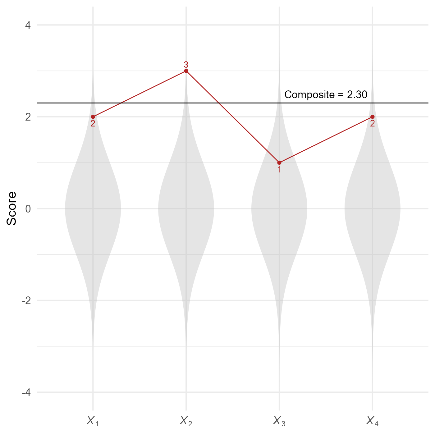
Suppose that there is a profile of scores in such that:
As seen in Figure 2, this profile of scores is summarized by a composite score of 2.30.

How can we calculate the Mahalanobis distance for profiles that all have the same elevation (i.e., composite score)? For your reference, we will do everything “by hand” using matrix algebra.
In r, we can make a named vector of scores like so:
X <- c(
  X_1 = 2,
  X_2 = 3,
  X_3 = 1,
  X_4 = 2
)

X
#> X_1 X_2 X_3 X_4
#>   2   3   1   2
We will need to store variable names:
We can create a matrix of factor loadings:
Now we calculate the model-implied correlations among the observed variables:
Presented formally, the model-implied correlations are:
We need to use this matrix to create a new 5 × 5 correlation matrix that includes the correlations among the four variables and also each variable’s correlation with the general composite score (i.e., the standardized sum of four variables). Fortunately, such a matrix can be calculated with only a few steps.
We will need a “weight” matrix that will select each variable individually and also the sum of the four variables.
Notice that the first column of this matrix has a 1 in first position and zeroes elsewhere. It selects the first variable, X1. The second column selects X2, and so on to the fourth column. The last column is all ones, which will select all four variables and add them up.
We can construct this matrix with the diag function, which creates an identity matrix. This matrix is appended to a column of ones:
Now we can use the weight matrix w to calculate the covariance matrix:
Now we need to convert the covariance matrix to a correlation matrix. With matrix equations, we would need to create a matrix of with a vector of variances on the diagonal:
Then we would take the square root, invert this matrix, and then pre-multiply it and post-multiply it by the covariance matrix.
If we really want to use pure matrix algebra functions, we could do this:
D_root_inverted <- Sigma %>%
  diag() %>%
  sqrt() %>%
  diag() %>%
  solve() %>%
  `rownames<-`(v_names) %>%
  `colnames<-`(v_names)

R_all <- D_root_inverted %*% Sigma %*% D_root_inverted

R_all
#>                   X_1       X_2       X_3       X_4 X_Composite
#> X_1         1.0000000 0.8550000 0.8075000 0.5700000   0.9294705
#> X_2         0.8550000 1.0000000 0.7650000 0.5400000   0.9086239
#> X_3         0.8075000 0.7650000 1.0000000 0.5100000   0.8863396
#> X_4         0.5700000 0.5400000 0.5100000 1.0000000   0.7533527
#> X_Composite 0.9294705 0.9086239 0.8863396 0.7533527   1.0000000
However, it is probably best to sidestep all this complication of converting covariances to correlations with the cov2cor function:
# Convert covariance matrix to correlations
R_all <- cov2cor(Sigma)

R_all
#>                   X_1       X_2       X_3       X_4 X_Composite
#> X_1         1.0000000 0.8550000 0.8075000 0.5700000   0.9294705
#> X_2         0.8550000 1.0000000 0.7650000 0.5400000   0.9086239
#> X_3         0.8075000 0.7650000 1.0000000 0.5100000   0.8863396
#> X_4         0.5700000 0.5400000 0.5100000 1.0000000   0.7533527
#> X_Composite 0.9294705 0.9086239 0.8863396 0.7533527   1.0000000
Calculate composite scores
To calculate the standardized composite score , add each variable’s deviation from its own mean and divide by the square root of the sum of the observed score covariance matrix.
Where
is a standardized composite score.
is a vector of observed scores.
is the vector of means for the variables.
is the covariance matrix of the variables.
is a vector of ones compatible with .
The composite score is:
# Population means of observed variables
mu_X <- rep_along(X, 0)

# Population standard deviations of observed variables
sd_X <- rep_along(X, 1)

# Covariance Matrix
Sigma_X <- diag(sd_X) %*% R_X %*% diag(sd_X)

# Vector of ones
ones <- rep_along(X, 1)

# Standardized composite score
z_C <- c(ones %*% (X - mu_X) / sqrt(ones %*% (Sigma_X) %*% ones))
Estimate expected test scores conditioned on a composite score
Given a particular composite score, we need to calculate a predicted score. That is, if the composite score is 1.5 standard deviations above the mean, what are the expected subtest scores?
Where
is the vector of expected subtest scores
is the vector of standard deviations for
is the composite score
is a vector of correlations of each variable in with the composite score
is the vector of means for
Thus,
# Predicted value of X, given composite score
X_hat <- sd_X * z_C * R_all[v_observed, v_composite] + mu_X
Calculating the Conditional Mahalanobis Distance
Where
is the Conditional Mahalanobis Distance
is a vector of subtest scores
is the vector of expected subtest scores
is the covariance matrix of the subtest scores
Suppose there are k outcome scores, and j composite scores used to calculate the expected scores . If multivariate normality of the subtest scores can be assumed, then the Conditional Mahalanobis Distance squared has a χ2 distribution with k − j degrees of freedom.
If we can assume that the observed variables in X are multivariate normal, a profile of X = {2,3,1,2} is more unusual than 96% of profiles that also have a composite score of zC = 2.3.