Recreating APA Manual Table 7.20 in R with apa7

Making tables in APA style (Part 20 of 24)

In this 24-part series, each of the tables in Chapter 7 of the Publication Manual of the American Psychological Association (7th Edition) is recreated with apa7, flextable, easystats, and tidyverse functions.

NoteHighlights

• Display of multilevel models

library(apa7)
library(flextable)
library(ftExtra)
library(tidyverse)
library(easystats)
library(lme4)
set_flextable_defaults(theme_fun = theme_apa, 
                       font.family = "Times New Roman")

Figure 1

Screenshot of the APA Manual’s Table 7.20

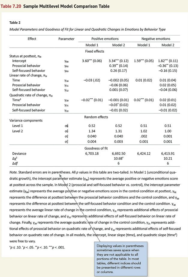
I wanted the experience of making the table close to what would happen in a real analysis. Instead of copying table’s text exactly, I simulated multilevel data based on the results in Figure 1. Although there are functions that can simulate multilevel data, In my experience, I can more easily get exactly what I want if I write out the equations and them simulate the data myself. The only information I lacked were the sample sizes at levels 1 and 2 and the number of times these behaviors were measured in the observational study. I supplied some numbers that made the models run without error.

Level 1

\begin{aligned} Y_{ij} &= b_{0j} + b_{1j}Time_{ij} + b_{2j}Time_{ij}^2 + e_{ij}\\ e_{ij}&\sim\mathcal{N}\left(0,\tau_1\right) \end{aligned}

Level 2

\begin{aligned} b_{0j} &= b_{00}+b_{01}PBS_j+b_{02}SFB_j+e_{0j}\\ b_{1j} &= b_{10}+b_{11}PBS_j+b_{12}SFB_j+e_{1j}\\ b_{2j} &= b_{20}+b_{21}PBS_j+b_{22}SFB_j+e_{2j}\\ e_2&=\begin{bmatrix} e_{0j}\\ e_{1j}\\ e_{2j} \end{bmatrix}\\ \tau_2&=\begin{bmatrix} \tau_{00}&0&0\\ 0&\tau_{11}&0\\ 0&0&\tau_{22}\\ \end{bmatrix}\\ e_2&\sim\mathcal{N}\left(0,\tau_2\right) \end{aligned}

Because of the stars after the coefficients, I was not able to find a good option for aligning both the coefficients and standard errors in the “Model” columns, so I aligned the coefficients only.

Getting coefficients, variance components, and fit statistics in the same table required a lot of custom formatting. Automating some of this would be a good idea.

set.seed(123)
# Number of people
n_2 <- 400
# Number of time points
n_1 <- 15

d_parameter <- tibble::tibble(
  symbol = c(
    "b_00", "b_01", "b_02",
    "b_10", "b_11", "b_12",
    "b_20", "b_21", "b_22",
    "s_e", "s_0", "s_1", "s_2"),
  Positive = c(
    3.34, 0.39, 0.26, -0.002, -0.06, 0.001,
    -0.001, -0.03, -0.01, 0.52, 1.31, 0.04, 0.03),
  Negative = c(
    1.82, -0.36, -0.16, 0.01, 0.02, -0.04, 0.02, 
    0.01, -0.01, 0.51, 1, 0.02, 0.02),
  Parameter = c(
     "(Intercept)",
     "PBS",
     "SFB",
     "Time",
     "PBS:Time",
     "Time:SFB",
     "I(Time^2)",
     "PBS:I(Time^2)",
     "I(Time^2):SFB",
     "SD (Observations)",
     "SD (Intercept)",
     "SD (Time)", 
     "SD (I(Time^2))"),
  pname = c(
    "Intercept",
    "Prosocial behavior",
    "Self-focused behavior",
    "Time",
    "Prosocial behavior", 
    "Self-focused behavior",
    "Time^2",
    "Prosocial behavior", 
    "Self-focused behavior",
    "Level 1",
    "Level 2",
    "Level 2",
    "Level 2"),
  l2 = c(
    rep("Status at postest, &pi;~0j~", 3),
    rep("Linear rate of change, &pi;~1j~", 3),
    rep("Quadratic rate of change, &pi;~2j~", 3),
    rep("Variance components", 4)),
  effect_type = c(
    rep("Fixed", 9),
    rep("Random", 4))
) |> 
  mutate(symbol = fct_inorder(symbol),
         pname = fct_inorder(pname))

# Level 1 variances
tau_1 <- d_parameter |> 
  filter(symbol == "s_e") |> 
  select(symbol, Positive, Negative) |>
  pivot_longer(-symbol) |> 
  select(name, value) |> 
  deframe()

# Level 2 variances
tau_2 <- d_parameter |> 
  filter(str_starts(symbol, "s_")) |> 
  filter(symbol != "s_e") |> 
  select(symbol, Positive, Negative) |>
  pivot_longer(-symbol) |>
  select(-symbol) |> 
  nest(value = -name) |> 
  mutate(value = map(
    value, 
    \(x) diag(unlist(x)))) |>
  deframe()

# Fixed effects
d_parameter_fixed <- d_parameter |> 
  filter(effect_type == "Fixed") |> 
  select(symbol, Positive, Negative) |> 
  pivot_longer(-symbol, 
               names_to = "dv", 
               values_to = "b") |>
  pivot_wider(names_from = symbol, 
              values_from = b)

# Level 2 simulated data
d_2 <- tibble(
  id = seq_len(n_2),
  Intercept = 1,
  PBS = rnorm(n_2),
  SFB = rnorm(n_2)
) |> 
  crossing(
    dv = fct_inorder(c("Positive", 
                       "Negative"))) |> 
  nest(data = -dv) |> 
    mutate(
      tau_2 = tau_2, 
      e_2 = map(
        tau_2, 
        \(x) {
          mvtnorm::rmvnorm(
            n = n_2, 
            mean = c(
              e_0j = 0, 
              e_1j = 0, 
              e_2j = 0), 
            sigma = x) |> 
            as_tibble()
        })) |> 
    select(-tau_2) |> 
    unnest(c(data, e_2)) |> 
  left_join(d_parameter_fixed, by = join_by(dv)) |> 
  mutate(b_0j = b_00 + b_01 * PBS + b_02 * SFB + e_0j,
         b_1j = b_10 + b_11 * PBS + b_12 * SFB + e_1j,
         b_2j = b_20 + b_21 * PBS + b_22 * SFB + e_2j)

# Level 1 simulated data
d_1 <- d_2 |> 
  crossing(
    Time = seq(0, n_1 - 1)
  ) |> 
  nest(data = -dv) |> 
  mutate(tau_1 = tau_1,
         e_ij = map2(tau_1, data, \(tau, d) {
           rnorm(nrow(d), sd = sqrt(tau))
           })) |> 
  unnest(c(data, e_ij)) |>
  mutate(
    y = b_0j + b_1j * Time + b_2j * Time^2 + e_ij) |> 
  select(dv, id, PBS, SFB, Time, y) 

# Analyze data
fit <- d_1 |> 
  nest(data = -dv) |> 
  mutate(
    `Model 1` = map(
      data, 
      \(d) {
        lmer(y ~ 1 + Time + I(Time^2) + 
               (1 + Time + I(Time^2) || id), 
             data = d)
      }),
    `Model 2` = map(
      data, 
      \(d) {
        lmer(y ~ 1 + PBS * Time + PBS * I(Time^2) + 
               SFB * Time + SFB * I(Time^2) + 
               (1 + Time + I(Time^2) || id), 
             data = d)
        })
      ) |> 
  select(-data) |> 
  pivot_longer(-c(dv), 
               names_to = "Model", 
               values_to = "fit") |> 
  mutate(
    parameters = map(
      fit, parameters::parameters, 
      include_sigma = TRUE))

# Peformance statistics
d_performance <- fit |> 
  select(dv, fit) |> 
  summarise(fit = list(fit), .by = dv) |> 
  mutate(p = map(fit, \(f1) {
    anova(f1[[1]], f1[[2]]) |> 
      as_tibble() |> 
      rename(Deviance = `-2*log(L)`, 
             deltachi2 = Chisq,
             df_diff = Df,
             p = `Pr(>Chisq)`) |> 
      mutate(Model = paste0("Model ", 1:2),
             chistar = p2stars(p),
             Deviance = align_chr(Deviance)) |> 
      select(
        Model, 
        Deviance, 
        deltachi2, 
        df_diff, 
        chistar) |> 
      apa_format_columns() |> 
      unite(`&Delta;&chi;^2^`, 
            `&Delta;&chi;^2^`, 
            chistar, 
            sep = "")
    })) |> 
  select(-fit) |> 
  arrange(desc(dv)) |> 
  unnest(p) |> 
  mutate(dv = paste0(dv, " emotions")) |>
  unite(dv, c(dv, Model)) |> 
  mutate(dv = fct_inorder(dv)) |> 
  pivot_longer(-dv, names_to = "Effect") |> 
  pivot_wider(names_from = dv) |> 
  mutate(effect_type = "Goodness of fit") |> 
  suppressMessages()
  
# Format data
d <- fit |> 
  unnest(parameters) |> 
  select(dv, Model, Parameter, Coefficient, SE, p) |> 
  mutate(Coefficient = align_chr(Coefficient)) |> 
  add_star_column(Coefficient, merge = TRUE) |> 
  mutate(SE = align_chr(SE, 
                                    accuracy = .01) |> 
           tagger(" (", ")"), 
         b = paste0(Coefficient, SE),
         dv = fct_inorder(paste(dv, "emotions"))) |> 
  select(dv, Model, Parameter, b) |> 
  unite(dv, c(dv, Model)) |> 
  pivot_wider(names_from = dv, values_from = b) |> 
  left_join(
    d_parameter |> 
      select(Parameter, 
             symbol, 
             pname, 
             l2, 
             effect_type), 
    by = join_by(Parameter)) |> 
  arrange(symbol) |> 
  rename(Effect = pname) |> 
  select(-Parameter) |> 
  relocate(Effect, symbol, .before = 0) |> 
  mutate(symbol = as.character(symbol) |> 
           str_replace_all(
             c(`s_` = "&sigma;~",
               `b_` = "&gamma;~")) |> 
           paste0("~", ifelse(
             str_detect(symbol, "^s"), 
             "^2^", 
             ""))) |> 
  mutate(Effect = as.character(Effect) |> str_replace("\\^2", "^2^")) |> 
  as_grouped_data(c("effect_type", "l2"))  |> 
  mutate(Effect = ifelse(is.na(l2), Effect, l2)) |> 
  select(-l2) |> 
  tidyr::fill(effect_type) |> 
  filter(!is.na(Effect))  |> 
  bind_rows(d_performance) |> 
  mutate(across(
    everything(), 
    \(x) replace_na(x, replace = ""))) |> 
  rename(`Parameter ` = symbol) 

# Make table
d |> 
  apa_flextable(
    row_title_column = effect_type, 
    row_title_align = "center",
    font_size = 10, 
    line_spacing = 1.5) |> 
  align(j = 1, i = ~is.na(row_title)) |> 
  padding(
    j = 1, 
    i = ~(is.na(row_title) & 
            `Parameter ` != ""), 
    padding.left = 15) |> 
  merge_v(j = "Effect") |> 
  width(width = c(1.70, .55, 
                  1.05, 1.05, .05, 
                  1.05, 1.05))

Table 1

Model Parameters and Goodness of Fit for Linear and Quadratic Changes in Emotions by Behavior Type

Effect	Parameter	Negative emotions			Positive emotions
		Model 1	Model 2		Model 1	Model 2
Fixed
Status at postest, π0j
Intercept	γ00	1.79*** (0.06)	1.80*** (0.06)		3.40*** (0.06)	3.39*** (0.06)
Prosocial behavior	γ01		−0.34*** (0.06)			0.25*** (0.06)
Self-focused behavior	γ02		−0.17** (0.06)			0.22*** (0.06)
Linear rate of change, π1j
Time	γ10	0.00 (0.01)	0.00 (0.01)		0.00 (0.01)	0.00 (0.01)
Prosocial behavior	γ11		0.02 (0.01)			−0.08*** (0.01)
Self-focused behavior	γ12		−0.04*** (0.01)			0.02 (0.01)
Quadratic rate of change, π2j
Time2	γ20	0.02** (0.01)	0.02** (0.01)		0.02 (0.01)	0.02 (0.01)
Prosocial behavior	γ21		0.00 (0.01)			−0.03*** (0.01)
Self-focused behavior	γ22		0.00 (0.01)			−0.02* (0.01)
Random
Variance components
Level 1	σe2	0.73	0.73		0.71	0.71
Level 2	σ02	1.08	1.01		1.15	1.11
	σ12	0.13	0.13		0.22	0.20
	σ22	0.13	0.13		0.18	0.18
Goodness of fit
Deviance		17,862.07	17,800.95		18,214.81	18,133.36
Δχ2			61.12***			81.45***
Δdf			6			6

Note. Standard errors are in parentheses. All p values in this table are two tailed. In Model 1 (unconditional quadratic growth), the intercept parameter estimate (γ₀₀) represents the average positive or negative emotions score at posttest across the sample. In Model 2 (prosocial and self-focused behavior vs. control), the intercept parameter estimate (γ₀₀) represents the average positive or negative emotions score in the control condition at posttest, γ₀₂ represents the difference at posttest between the prosocial behavior conditions and the control condition, and γ₀₃ represents the difference at posttest between the self-focused behavior condition and the control condition. γ₁₀ represents the average linear rate of change in the control condition, γ11 represents additional effects of prosocial behavior on linear rate of change, and γ₁₂ represents additional effects of self-focused behavior on linear rate of change. Finally, γ₂₀ represents the average quadratic rate of change in the control condition, γ₂₁ represents additional effects of prosocial behavior on quadratic rate of change, and γ₂₂ represents additional effects of self-focused behavior on quadratic rate of change. In all models, the intercept, linear slope (time), and quadratic slope (time2) were free to vary.

^* p < .05. ^** p < .01. ^*** p < .001.

• First
• Previous
• Next
• Last