Recreating APA Manual Table 7.15 in R with apa7

Making tables in APA style (Part 15 of 24)

In this 24-part series, each of the tables in Chapter 7 of the Publication Manual of the American Psychological Association (7th Edition) is recreated with apa7, flextable, easystats, and tidyverse functions.

NoteHighlights

• Automatic formatting of lm (linear model) analyses with apa_performance and apa_compare_performance.

library(apa7)
library(flextable)
library(ftExtra)
library(tidyverse)
library(easystats)
set_flextable_defaults(theme_fun = theme_apa, 
                       font.family = "Times New Roman")

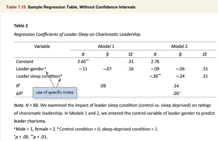
Figure 1

Screenshot of the APA Manual’s Table 7.15

I love the easystats ecosystem. It provides a coherent framework for data-analysts to process and display statistical analyses. It makes so many previously tedious things simple. However, it was not specifically designed for the final display of APA tables. The apa7 package has a few functions and features that help process the output of easystats functions to make them table-ready.

First, lets simulate some data that resembles the data underlying the models in Figure 1, and create regression models for Models 1 and 2.

set.seed(1)
# sample size
n <- 88

# simulated data
d <- tibble(
  leader_gender = sample(0:1, n, replace = TRUE),
  leader_sleep_condition = sample(0:1, 88, replace = TRUE),
  charisma = 2.76 - .09 * leader_gender - 
    .36 * leader_sleep_condition + 
    rnorm(n, sd = 0.5))

# Models 1 and 2
m1 <- lm(charisma ~ leader_gender, data = d)
m2 <- lm(charisma ~ leader_gender + leader_sleep_condition, data = d)

The parameters::parameters function from the easystats ecosystem displays information about regression predictors.

parameters(m2) 

Parameter              | Coefficient |   SE |         95% CI | t(85) |      p
-----------------------------------------------------------------------------
(Intercept)            |        2.79 | 0.08 | [ 2.62,  2.95] | 33.17 | < .001
leader gender          |       -0.20 | 0.10 | [-0.40,  0.00] | -1.96 | 0.054 
leader sleep condition |       -0.34 | 0.10 | [-0.55, -0.14] | -3.37 | 0.001 

Uncertainty intervals (equal-tailed) and p-values (two-tailed) computed
  using a Wald t-distribution approximation.

That is a really nice display. However, if we convert it directly with flextable, we get something far less polished.

parameters(m2) |> 
  flextable()

Parameter	Coefficient	SE	CI	CI_low	CI_high	t	df_error	p
(Intercept)	2.79	0.08	0.95	2.62	2.95	33.17	85	0.00
leader_gender	-0.20	0.10	0.95	-0.40	0.00	-1.96	85	0.05
leader_sleep_condition	-0.34	0.10	0.95	-0.55	-0.14	-3.37	85	0.00

As it turns out, the output of the parameters function undergoes a fair bit of processing before it prints. The output is a data.frame with a parameters_model class and many attributes that can be used by the easystats formatting functions. If we want to see the underlying data, we can convert the output to a data.frame or tibble.

parameters(m2) |> 
  as_tibble()

# A tibble: 3 × 9
  Parameter     Coefficient     SE    CI CI_low  CI_high     t df_error        p
  <chr>               <dbl>  <dbl> <dbl>  <dbl>    <dbl> <dbl>    <int>    <dbl>
1 (Intercept)         2.79  0.0840  0.95  2.62   2.95    33.2        85 2.05e-50
2 leader_gender      -0.200 0.102   0.95 -0.402  0.00312 -1.96       85 5.36e- 2
3 leader_sleep…      -0.344 0.102   0.95 -0.547 -0.141   -3.37       85 1.13e- 3

If we really want just the output of parameters as it displays, we use the insight::format_table function.

parameters(m2, ci = .95) |> 
  insight::format_table() 

               Parameter Coefficient   SE         95% CI t(85)      p
1            (Intercept)        2.79 0.08 [ 2.62,  2.95] 33.17 < .001
2          leader gender       -0.20 0.10 [-0.40,  0.00] -1.96 0.054 
3 leader sleep condition       -0.34 0.10 [-0.55, -0.14] -3.37 0.001 

This gets us closer to APA style, but not quite all way there. We would like things to be nearly automatic and yet be able to fine-tune the output. Behold!

apa_parameters(m2) 

# A tibble: 3 × 6
  Variable               `*B*` `*SE*` `β` `*t*(85)` `*p*`
  <chr>                  <chr> <chr>  <chr>    <chr>     <chr>
1 Constant                2.79 0.08    .00     33.17     <.001
2 Leader Gender          −0.20 0.10   −.20     −1.96      .05 
3 Leader Sleep Condition −0.34 0.10   −.34     −3.37      .001

The apa_parameters function is a wrapper around the parameters function with defaults that produce APA style output via markdown syntax. The columns are decimal aligned, statistics are italicized, the intercept is called a “Constant”, and the variable names are printed in title case.

Applying apa_flextable to the output gives us perfect APA style:

apa_parameters(m2) |> 
  apa_flextable() 

Variable	B	SE	β	t(85)	p
Constant	2.79	0.08	.00	33.17	<.001
Leader Gender	−0.20	0.10	−.20	−1.96	.05
Leader Sleep Condition	−0.34	0.10	−.34	−3.37	.001

The apa_format_columns function and a few others like apa_parameters, apa_performance, and apa_compare_performance can process the output of the lm function.

Getting the output of apa_parameters and apa_compare_performance into the same table requires a rather complex process. Eventually I’d like to automate some of these steps.

# pf <- column_formats()
# pf$SE@header <- "*SE*"

m <- list(`Model 1` = m1, 
          `Model 2` = m2) 

d_parameters <- apa_parameters(
  m, 
  predictor_parameters = c(
    "Coefficient", 
    "Std_Coefficient", 
    "SE"))

d_performance <- apa_performance_comparison(
  m,
  metrics = c("R2", "deltaR2"),
  starred = "deltaR2") |> 
  pivot_longer(-Model, names_to = "Variable") |> 
  mutate(Model = paste0(Model, "_&beta;")) |> 
  pivot_wider(names_from = Model)

d_parameters |> 
  pivot_wider_name_first(
    id_cols = Variable, 
    names_from = Model, 
    values_from = 3:5) |> 
  mutate(Variable = str_to_sentence(Variable)) |>
  add_row(d_performance) |>
  mutate(across(-Variable, \(x) align_chr(
    x,
    center = "\\.", 
    side = "left",
    NA_value = "") |> 
      star_balance())) |> 
  apa_flextable(no_format_columns = Variable) |> 
  align(j = 1, align = "left") |> 
  flextable::add_footer_lines(values = as_paragraph_md("*Note*. *N*&nbsp;=&nbsp;88. We examined the impact of leader sleep condition (control vs. sleep deprived) on ratings of charismatic leadership. In Models 1 and 2, we entered the control variable of leader gender to predict leader charisma.")) |> 
  footnote(i = 2, 
           j = 1, 
           value = as_paragraph("Male = 1, female = 2. "), 
           ref_symbols = "a ") |>
    footnote(i = 3, 
             j = 1, 
             value = as_paragraph(
               "Control condition = 0, sleep-deprived condition = 1"), 
             ref_symbols = "b ", 
             inline = T, 
             sep = ".") |> 
  add_footer_lines(
    values = as_paragraph_md("\\* *p* < .05. \\*\\* *p* < .01.")) |> 
  align(align = "left", part = "footer")

Table 1

Regression Coefficients of Leader Sleep on Charismatic Leadership

Variable	Model 1				Model 2
	B	β	SE		B	β	SE
Constant	2.65	.00	0.08		2.79	.00	0.08
Leader gendera	−0.24	−.23	0.11		−0.20	−.20	0.10
Leader sleep conditionb					−0.34	−.34	0.10
R2		.06				.17
ΔR2						.11**
Note. N = 88. We examined the impact of leader sleep condition (control vs. sleep deprived) on ratings of charismatic leadership. In Models 1 and 2, we entered the control variable of leader gender to predict leader charisma.
a Male = 1, female = 2. b Control condition = 0, sleep-deprived condition = 1.
* p < .05. ** p < .01.

• First
• Previous
• Next
• Last