Recreating APA Manual Table 7.18 in R with apa7

Making tables in APA style (Part 18 of 24)

In this 24-part series, each of the tables in Chapter 7 of the Publication Manual of the American Psychological Association (7th Edition) is recreated with apa7, flextable, easystats, and tidyverse functions.

NoteHighlights

• Presenting a sequence of regression models

library(apa7)
library(flextable)
library(ftExtra)
library(tidyverse)
library(easystats)
library(lavaan)
set_flextable_defaults(theme_fun = theme_apa, 
                       font.family = "Times New Roman")

Figure 1

Screenshot of the APA Manual’s Table 7.18

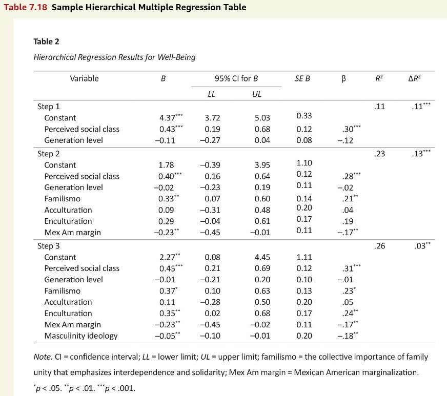
To make the conversion of analysis to table more realistic, I simulated data to resemble the Step 3 model.

```{r}
#| label: tbl-718
#| tbl-cap: "Hierarchical Regression: Results for Well-Being"
#| apa-note: 
#|   - "CI = confidence interval; *LL* = lower limit; 
#|   *UL* = upper limit; familismo = the collective 
#|   importance of family unity that emphasizes interdependence
#|   and solidarity; Mex Am margin = Mexican 
#|   American marginalization."
#|   - "^\\*^*p* < .05. ^\\*\\*^*p* < .01. ^\\*\\*\\*^*p* < .001."
set.seed(123)
# Make coefficients
d_coefficients <- tibble::tribble(
  ~Step,                ~Variable, ~beta,    ~b,
     1L, "Perceived social class",  0.31,  0.45,
     1L,       "Generation level", -0.01, -0.01,
     2L,              "Familismo",  0.23,  0.37,
     2L,          "Acculturation",  0.05,  0.11,
     2L,          "Enculturation",  0.24,  0.35,
     2L,        "Mex {Am} margin", -0.17, -0.23,
     3L,   "Masculinity ideology", -0.18, -0.05
  ) |> 
  mutate(vname = snakecase::to_any_case(
    Variable, 
    case = "parsed") |> fct_inorder(),
    Variable = fct_inorder(Variable))

# Make data
d <- d_coefficients |> 
  unite(vname, c(beta, vname), 
        sep = " * ") |> 
  pull(vname) |> 
  paste(collapse = " + ") |> 
  {
    \(x) paste0("y ~ ", x)
    }() |> 
  simulateData(standardized = TRUE, sample.nobs = 125) |> 
  mutate(y = y + 4) |> 
  as_tibble()

# Rescale data
for (i in seq_len(nrow(d_coefficients))) {
  d[,d_coefficients[i,]$vname] <- d[,d_coefficients[i,]$vname] * 
    d_coefficients[i,]$beta / 
    d_coefficients[i,]$beta
}

# Analyze data
d_analysis <- d_coefficients |>
  select(Step, vname) |>
  crossing(Model = 1:3) |>
  arrange(Model, Step) |>
  filter(Step <= Model) |>
  select(-Step) |>
  summarise(f = paste0(vname, collapse = " + "), 
            .by = Model) |>
  mutate(
    eq = paste0("y ~ ", f) |> map(formula),
    fit = map(eq, lm, data = d),
    Model = paste("Model", Model)
  )

# Format data
d_formatted <- d_analysis |>
  mutate(
    parameters = map(fit, model_parameters),
    std_parameters = map(fit, 
                         model_parameters, 
                         standardize  = "basic") |> 
      map(\(d) select(d, Std_Coefficient))
  ) |>
  select(Model, parameters, std_parameters) |>
  unnest(c(parameters, std_parameters)) |>
  select(-CI, -t, -df_error) |>
  rename(pp = p) |>
  relocate(SE, .before = Std_Coefficient) |>
  apa_format_columns() |>
  rename(`95% CI for *B*_*LL*` = LL,
         `95% CI for *B*_*UL*` = UL) |>
  as_grouped_data("Model") |>
  left_join(
    d_analysis |>
      pull(fit) |>
      apa_performance_comparison(
        starred = "deltaR2", 
        metrics = c("R2", "deltaR2")),
    by = join_by(Model)
  ) |>
  replace_na(list(Model = "", Variable = "")) |>
  unite(Variable, c(Variable, Model), sep = "") |>
  mutate(`&beta;` = ifelse(Variable == "Constant", NA, `&beta;`)) |> 
  add_star_column(c(`*B*`, `&beta;`), p = pp) |> 
  select(-pp) |>
  mutate(Variable = str_replace(Variable, "^Model", "Step") |> 
           snakecase::to_sentence_case() |> 
           str_replace(" am ", " Am "))

# Make table
d_formatted |> 
  apa_flextable(line_spacing = 1.5, 
                layout = "fixed") |>
  padding(i = ~!is.na(`*B*`), 
          j = 1, 
          padding.left = 15) |>
  surround(i = ~is.na(`*B*`), 
           border.top = fp_border_default(color = "gray30")) |> 
  width(width = 6.5 * c(3, .6, .4, 1, 1, 1, 
                           .6, .4, 1, 1) / 10)
```

Table 1

Hierarchical Regression: Results for Well-Being

Variable	B		95% CI for B		SE	β		R2	ΔR2
			LL	UL
Step 1								.03
Constant	4.00	***	3.85	4.16	0.08
Perceived Social Class	0.15		−0.01	0.30	0.08	.16
Generation Level	−0.04		−0.19	0.11	0.08	−.04
Step 2								.16	.13***
Constant	4.03	***	3.89	4.18	0.07
Perceived Social Class	0.19	*	0.04	0.34	0.08	.21	*
Generation Level	−0.04		−0.18	0.10	0.07	−.05
Familismo	0.18	*	0.03	0.32	0.07	.21	*
Acculturation	0.06		−0.09	0.22	0.08	.07
Enculturation	0.09		−0.06	0.24	0.08	.10
Mex Am Margin	−0.23	**	−0.38	−0.08	0.08	−.26	**
Step 3								.23	.06**
Constant	4.03	***	3.89	4.17	0.07
Perceived Social Class	0.18	*	0.03	0.32	0.07	.20	*
Generation Level	−0.08		−0.22	0.06	0.07	−.09
Familismo	0.18	*	0.04	0.32	0.07	.21	*
Acculturation	0.06		−0.09	0.21	0.07	.07
Enculturation	0.09		−0.06	0.24	0.07	.10
Mex Am Margin	−0.22	**	−0.37	−0.08	0.07	−.26	**
Masculinity Ideology	−0.22	**	−0.37	−0.08	0.07	−.26	**

Note. CI = confidence interval; LL = lower limit; UL = upper limit; familismo = the collective importance of family unity that emphasizes interdependence and solidarity; Mex Am margin = Mexican American marginalization.

^*p < .05. ^**p < .01. ^***p < .001.

• First
• Previous
• Next
• Last