Recreating APA Manual Table 7.10 in R with apa7

Making tables in APA style (Part 10 of 24)

In this 24-part series, each of the tables in Chapter 7 of the Publication Manual of the American Psychological Association (7th Edition) is recreated with apa7, flextable, easystats, and tidyverse functions.

NoteHighlights

• Correlation matrices and descriptive statistics with apa_cor

library(apa7)
library(flextable)
library(ftExtra)
library(tidyverse)
set_flextable_defaults(theme_fun = theme_apa, 
                       font.family = "Times New Roman")

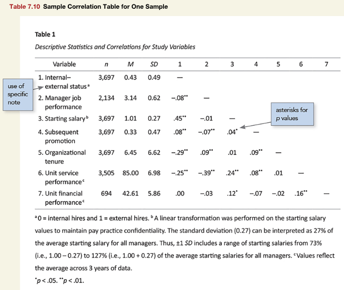
Figure 1

Screenshot of the APA Manual’s Table 7.10

The apa_cor function does a lot under the hood. By default, it gives the mean and standard deviation of each variable. By supplying a list of summary functions summary_functions = c("n", "M", "SD"), we can get the n for each variable, too.

set.seed(1234)

# Descriptives
d <- tibble::tribble(
                     ~Variable,    ~n,    ~M,  ~SD,
    "Internal--external status", 3697L,  0.43, 0.49,
     "Manager job performance", 2134L,  3.14, 0.62,
             "Starting salary", 3697L,  1.01, 0.27,
        "Subsequent promotion", 3697L,  0.33, 0.47,
         "Organization tenure", 3697L,  6.45, 6.62,
    "Unit service performance", 3505L,    85, 6.98,
  "Unit financial performance",  694L, 42.61, 5.86
  )

# Correlations
R <- "
r       1       2       3       4       5       6       7   
1   0.00    0.00    0.00    0.00    0.00    0.00    0.00
2   -0.08   0.00    0.00    0.00    0.00    0.00    0.00
3   0.45    -0.01   0.00    0.00    0.00    0.00    0.00
4   0.08    -0.07   0.04    0.00    0.00    0.00    0.00
5   -0.29   0.09    0.01    0.09    0.00    0.00    0.00
6   0.25    -0.39   0.24    0.08    0.01    0.00    0.00
7   0.00    0.03    0.12    -0.07   -0.02   0.16    0.00" |> 
    readr::read_tsv() |> 
  suppressMessages() |> 
    tibble::column_to_rownames("r") |> 
    as.matrix() |> 
  `dimnames<-`(list(d$Variable, d$Variable)) 

# Make R symmetric and fill diagonal with 1s
R <- (R + t(R)) |> `diag<-`(1)

# Make data
d_simulated <- mvtnorm::rmvnorm(
  n = max(d$n), 
  mean = deframe(d |> select(Variable, M)),
  sigma = diag(d$SD) %*% R %*% diag(d$SD)) |> 
  as_tibble() |> 
  map2_df(d$n, \(x, n) {
    k <- length(x)
    x[sample(1:k, size = k - n)] <- NA
    x
  }) |> 
  rename_with(hanging_indent, width = 15, indent = 0)


# Make table
d_simulated |> 
  apa_cor(
    summary_functions = c("n", "M", "SD"), 
    significance_note = FALSE, 
    p_value = c(.05, .01)) |>   
  footnote(
    i = 1, 
    j = "Variable", 
    value = as_paragraph(
      "0 = internal hires and 1 = external hires."), 
    ref_symbols = "a ",
    inline = TRUE, 
    sep = " ") |> 
  footnote(
    i = 3, 
    j = "Variable", 
    value = as_paragraph(
      paste("A linear transformation was performed on",
      "the starting salary values to maintain pay practice",
      "confidentiality. The standard deviation (0.27) can",
      "be interpreted as 27% of the average starting salary",
      "for all managers. Thus, ±1 SD includes a range of",
      "starting salaries from 73% (i.e., 1.00 – 0.27) to",
      "127% (i.e., 1.00 + 0.27) of the average starting",
      "salaries for all managers.")), 
    ref_symbols = "b ", 
    inline = TRUE, 
    sep = " ") |> 
  footnote(
    i = c(6,7), 
    j = "Variable", 
    value = as_paragraph(
      "Values reflect the average across 3 years of data."), 
    ref_symbols = "c ", 
    inline = TRUE, 
    sep = " ") |> 
  add_footer_lines(
    as_paragraph_md(
      "^\\*&numsp;^*p* < .05. ^\\*\\*&numsp;^*p* < .01."))

Table 1

Descriptive Statistics and Correlations for Study Variables

Variable		n	M	SD	1		2		3		4		5		6		7
1.	Internal– external statusa	3,697	0.43	0.48	—
2.	Manager job performance	2,134	3.12	0.61	−.08	**	—
3.	Starting salaryb	3,697	1.01	0.27	.47	**	−.02		—
4.	Subsequent promotion	3,697	0.33	0.47	.08	**	−.07	**	.05	**	—
5.	Organization tenure	3,697	6.51	6.65	−.27	**	.08	**	.03	*	.12	**	—
6.	Unit service performancec	3,505	84.92	6.92	.25	**	−.35	**	.25	**	.08	**	.02		—
7.	Unit financial performancec	694	42.29	5.84	−.02		.07		.05		−.09	*	−.01		.11	**	—
a 0 = internal hires and 1 = external hires. b A linear transformation was performed on the starting salary values to maintain pay practice confidentiality. The standard deviation (0.27) can be interpreted as 27% of the average starting salary for all managers. Thus, ±1 SD includes a range of starting salaries from 73% (i.e., 1.00 – 0.27) to 127% (i.e., 1.00 + 0.27) of the average starting salaries for all managers. c Values reflect the average across 3 years of data.
* p < .05. ** p < .01.

• First
• Previous
• Next
• Last