Segments • ggdiagram

Setup

Packages

library(ggdiagram)
library(ggplot2)
library(dplyr)
#> 
#> Attaching package: 'dplyr'
#> The following objects are masked from 'package:stats':
#> 
#>     filter, lag
#> The following objects are masked from 'package:base':
#> 
#>     intersect, setdiff, setequal, union
library(ggtext)
library(ggarrow)
library(arrowheadr)

Base Plot

To avoid repetitive code, we make a base plot:

my_font <- "Roboto Condensed"
my_font_size <- 20
my_point_size <- 2

# my_colors <- viridis::viridis(2, begin = .25, end = .5)
my_colors <- c("#3B528B", "#21908C")

theme_set(
  theme_minimal(base_size = my_font_size, base_family = my_font) +
    theme(axis.title.y = element_text(angle = 0, vjust = 0.5))
)

bp <- ggdiagram(
  font_family = my_font,
  font_size = my_font_size,
  point_size = my_point_size,
  linewidth = .5,
  theme_function = theme_minimal,
  axis.title.x =  element_text(face = "italic"),
  axis.title.y = element_text(
    face = "italic",
    angle = 0,
    hjust = .5,
    vjust = .5
  )
) +
  scale_x_continuous(labels = signs_centered, limits = c(-4, 4)) +
  scale_y_continuous(labels = signs::signs, limits = c(-4, 4))

Specifying a segment

A segment is a portion of a line between two points.

p1 <- ob_point(-3, -1)
p2 <- ob_point(3, 3)
s1 <- ob_segment(p1, p2)

bp + s1 + p1 + p2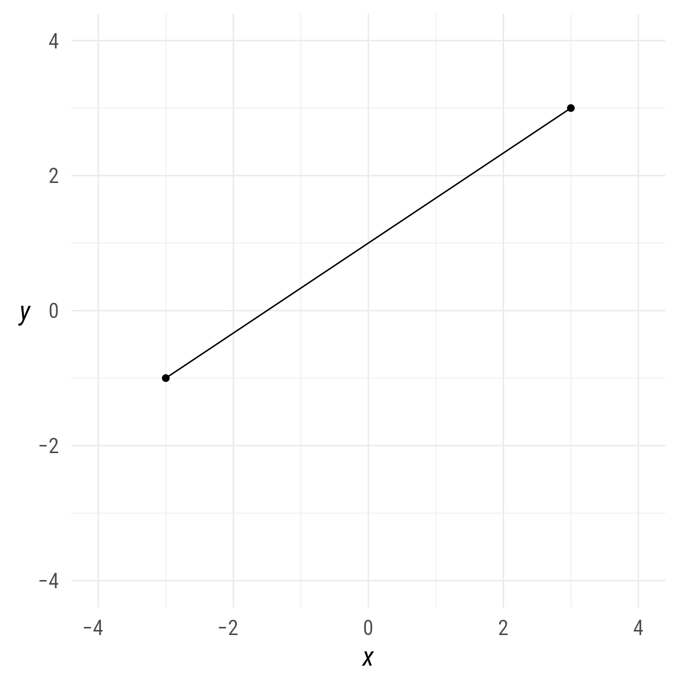

Figure 1: Plotting a segment and its endpoints

Features of a segment

Distance between points

s1@distance
#> [1] 7.211103

Alternately:

distance(s1)
#> [1] 7.211103

Line passing through the segment

The line that passes through the segment contains information about the segment, such as its slope, intercept, or angle.

To access the line that passes between both points:

s1@line
#> 
#> ── <ob_line>
#> # A tibble: 1 × 6
#>   slope intercept xintercept     a     b     c
#>   <dbl>     <dbl>      <dbl> <dbl> <dbl> <dbl>
#> 1 0.667         1       -1.5    -4     6    -6
s1@line@slope
#> [1] 0.6666667
s1@line@intercept
#> [1] 1
s1@line@angle
#> [1] "34°"

Code

bp +
  s1@line |> set_props(color = "royalblue4") +
  s1@midpoint(position = c(0, 1))@label(
    polar_just = ob_polar(s1@line@angle + degree(90), 1.5),
    plot_point = TRUE) +
  ob_label(c(equation(s1@line),
             paste0("Distance = ",
                    round(s1@distance, 2))),
           center = midpoint(s1),
           vjust = c(-.2, 1.1),
           angle = s1@line@angle)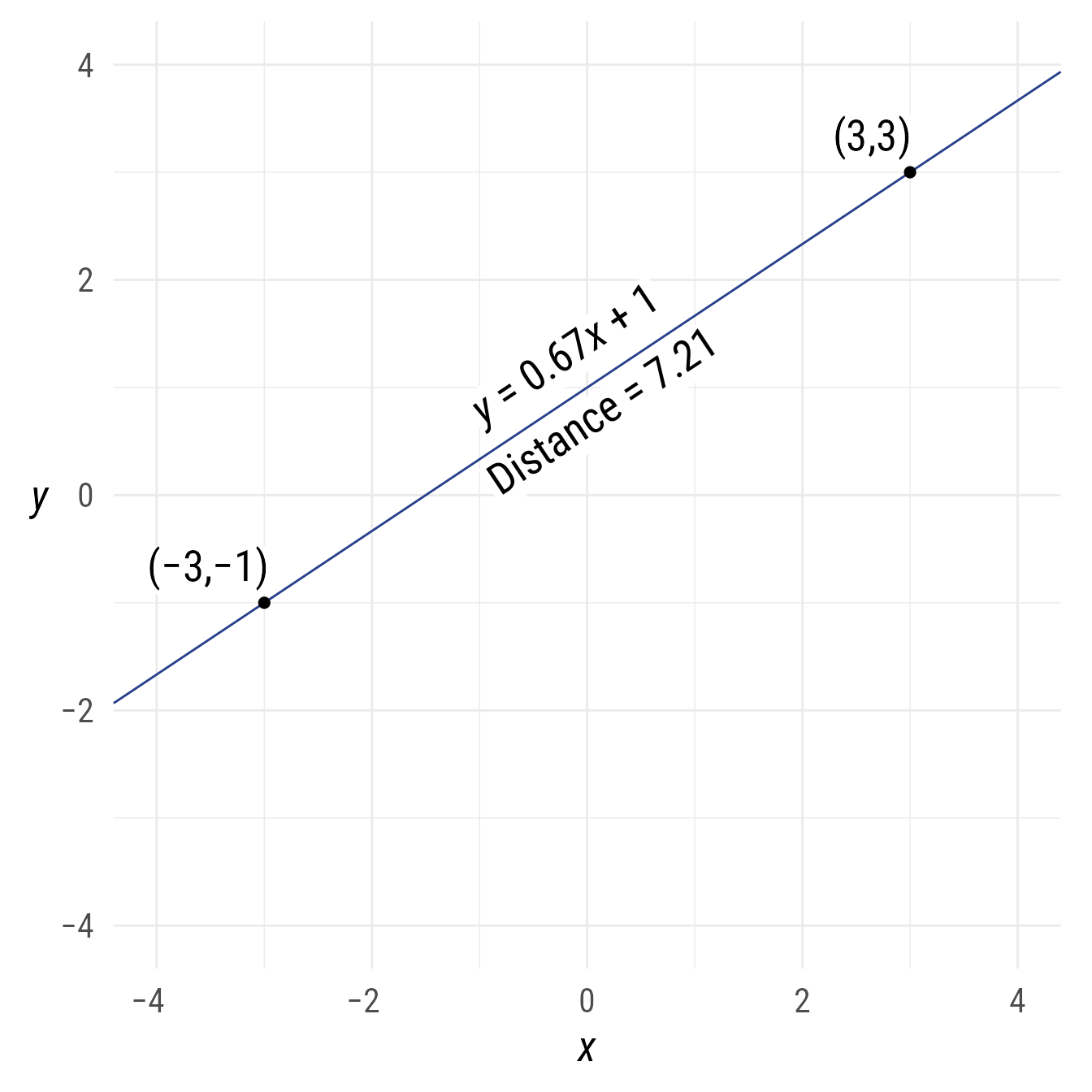

Midpoints

By default, the midpoint function’s position argument is .5, which finds the point halfway between the point of a segment:

s1@midpoint()
#> 
#> ── <ob_point>
#> # A tibble: 1 × 2
#>       x     y
#>   <dbl> <dbl>
#> 1     0     1

Code

bp +
  s1 +
  s1@midpoint()@label("Midpoint", hjust = 0, vjust = 1) +
  s1@midpoint(c(0, .5, 1))@label(
    plot_point = TRUE,
    hjust = 1,
    vjust = 0)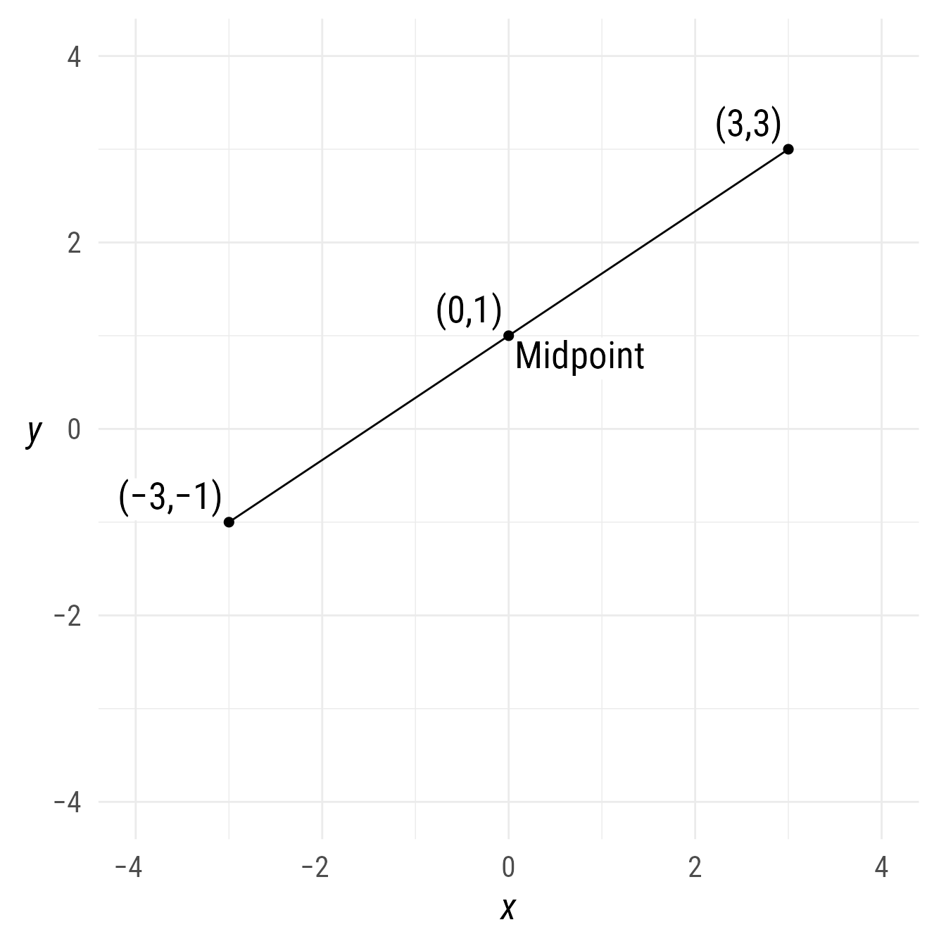

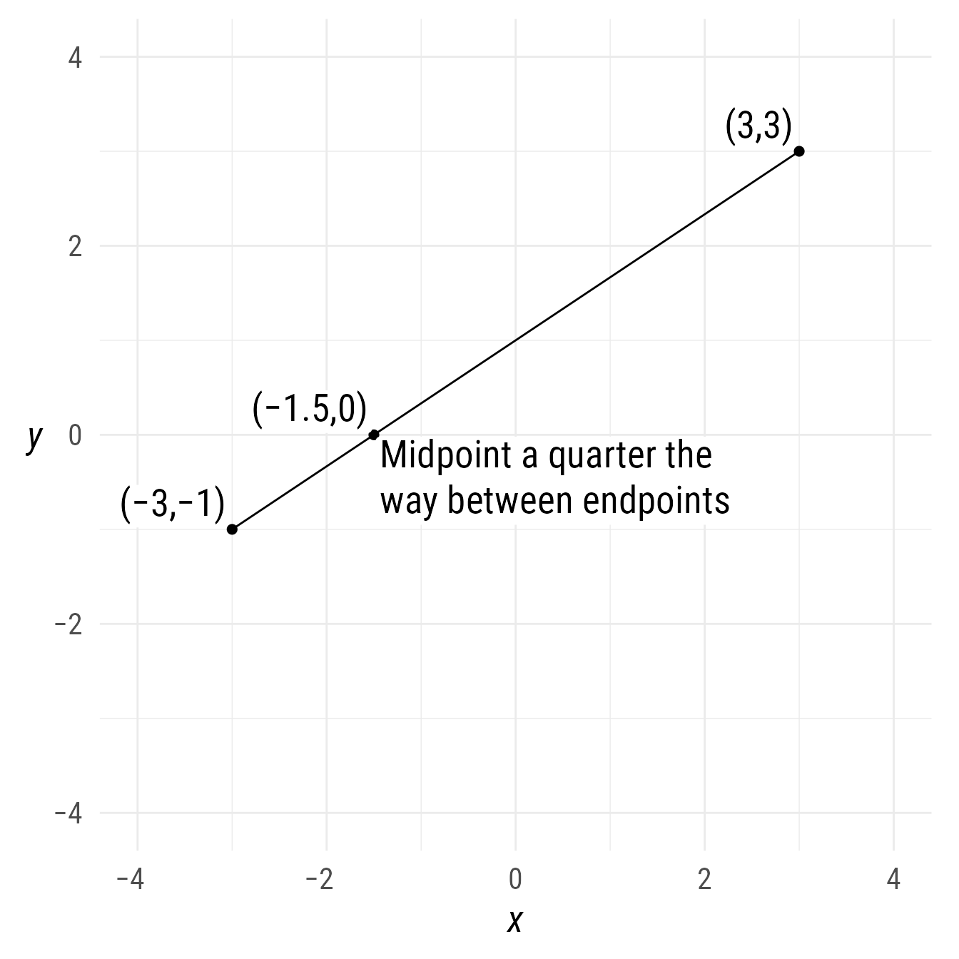
To find the midpoint 25% of the distance between the endpoints of segment:

s1@midpoint(position = .25)
#> 
#> ── <ob_point>
#> # A tibble: 1 × 2
#>       x     y
#>   <dbl> <dbl>
#> 1  -1.5     0

Code

bp +
  s1 +
  {p25 <- s1@midpoint(.25)} +
  p25@label(
    label = c(
      p25@auto_label,
      "Midpoint a quarter the<br>way between endpoints"
    ),
    vjust = c(0, 1),
    hjust = c(1, 0)
  ) +
  s1@midpoint(c(0, 1))@label(plot_point = TRUE,
                             hjust = 1,
                             vjust = 0)

Multiple midpoints can be specified:

bp +
  s1 +
    s1@midpoint(seq(0, 1, .2))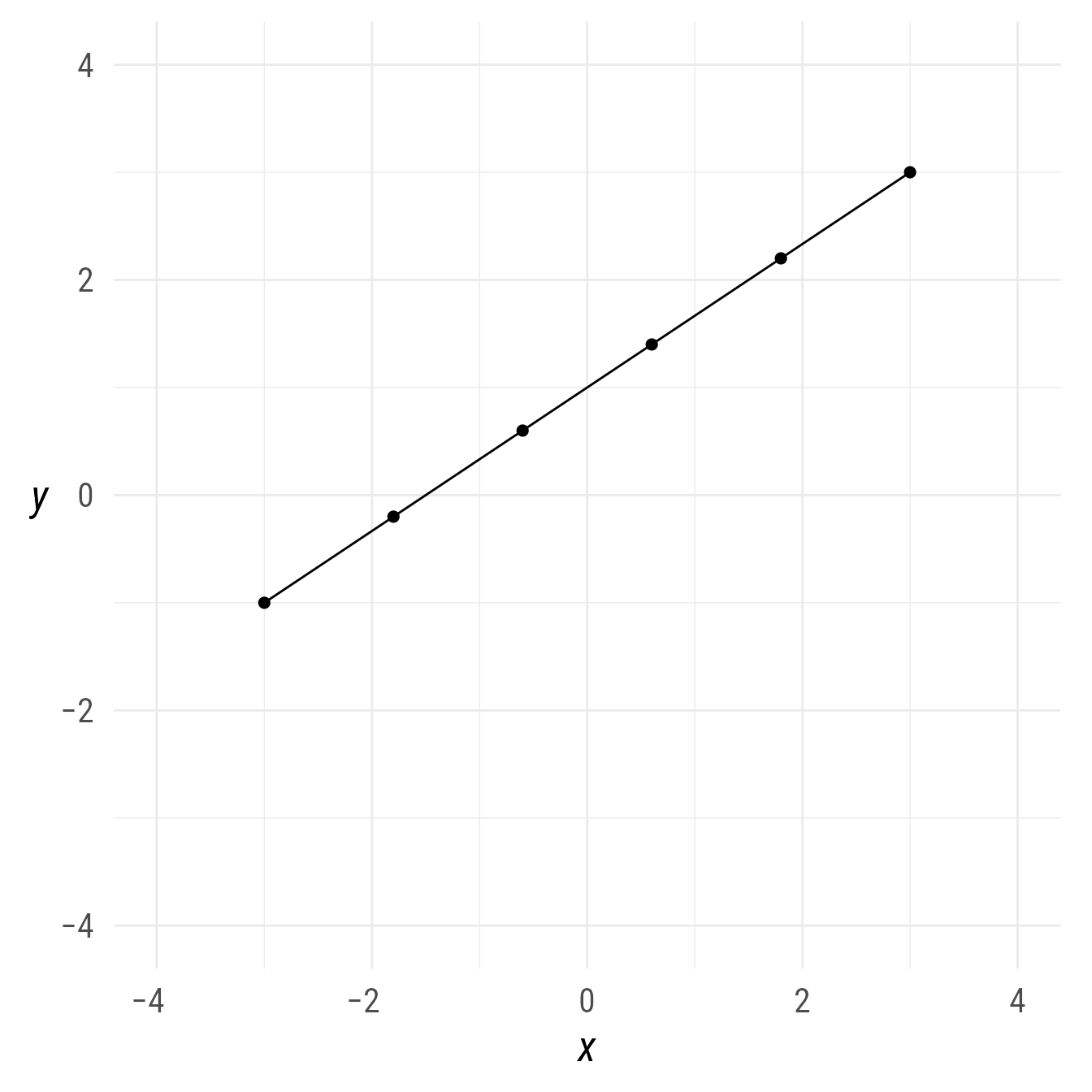

A quick way to get the endpoints of a segment is to specify “midpoints” at positions 0 and 1:

bp +
  s1 +
  s1@midpoint(c(0, 1))

Figure 6: Selecting a segment’s endpoints via the `midpoint` property.

Segment chains

If a point object with multiple points is placed in the p1 slot but the p2 slot is left empty, a series of segments chained together will be created.

bp +
  ob_segment(
    ob_point(x = c(-4, -2, -1, 2, 4),
             y = c(-2, 1, -2, 3, -3)))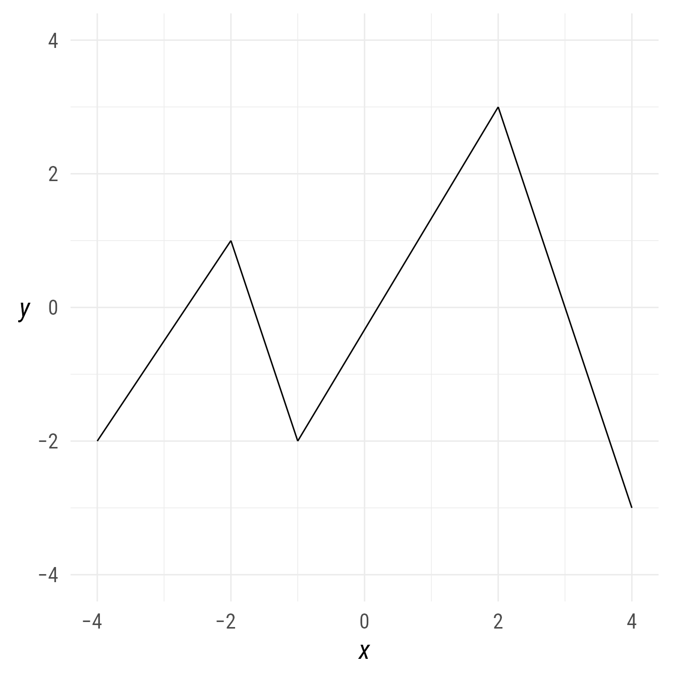

Arrowheads and fins

In the ob_segment function, the arrow_head and arrow_fins arguments can be set with any arrowhead function from the ggarrow or the arrowheadr packages. Any 2-column matrix will also be acceptable, as shown here. The default arrowhead can be used via the arrowhead() function. The size of the arrowhead and fins can also be controlled independently with the length_head and length_fins arguments.

bp + ob_segment(p1, p2, 
                arrow_head = arrowhead(), 
                arrow_fins = ggarrow::arrow_fins_feather(), 
                length_head = 5,
                length_fins = 7, 
                linewidth = 2)

Labeling segments

By default, any label is set at the midpoint of the segment (see Figure 9). If it is plain text, it will be just above the segment. Its angle will match that of the segment, but this can be turned off by setting label_sloped to FALSE.

bp + ob_segment(p1, p2, label = "My label")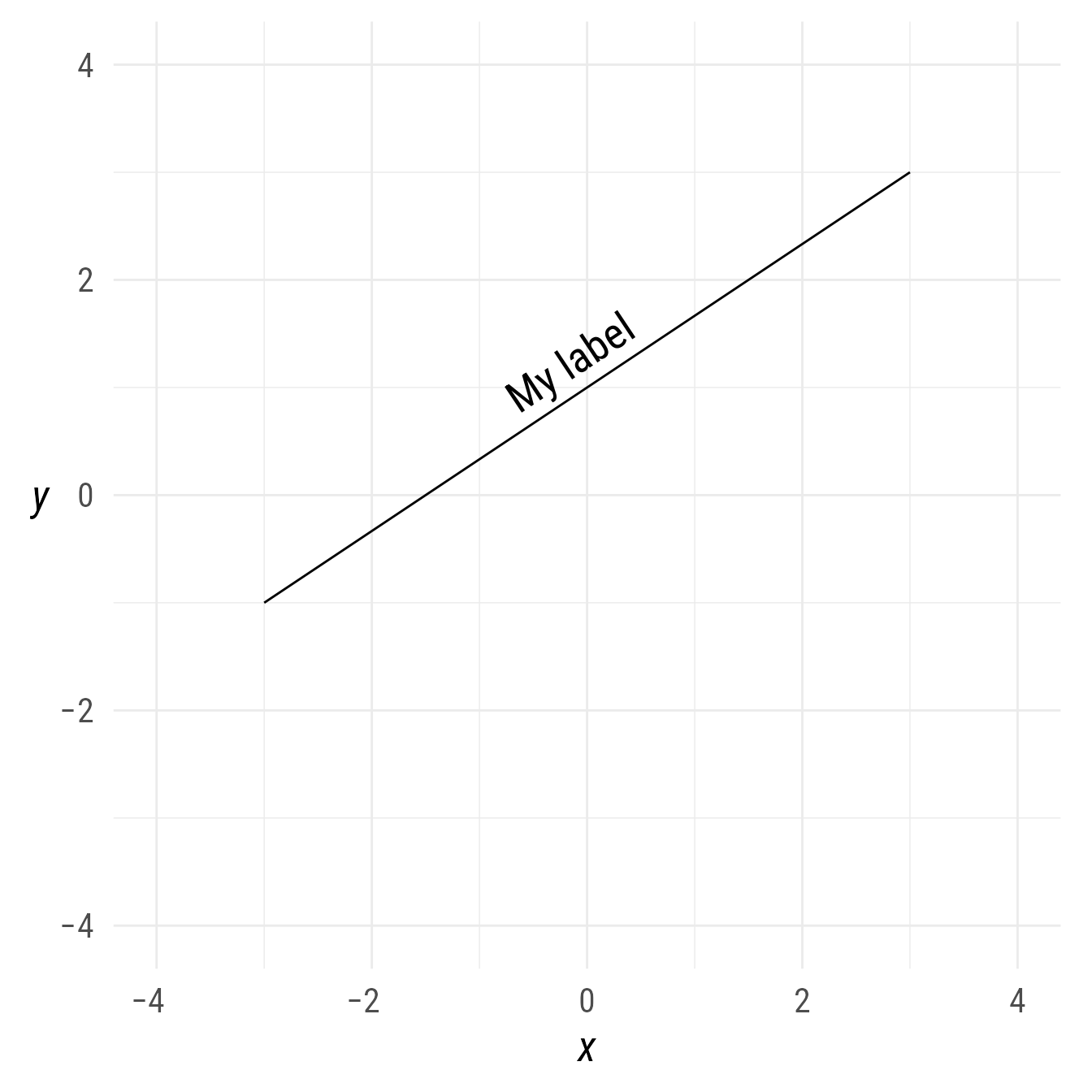

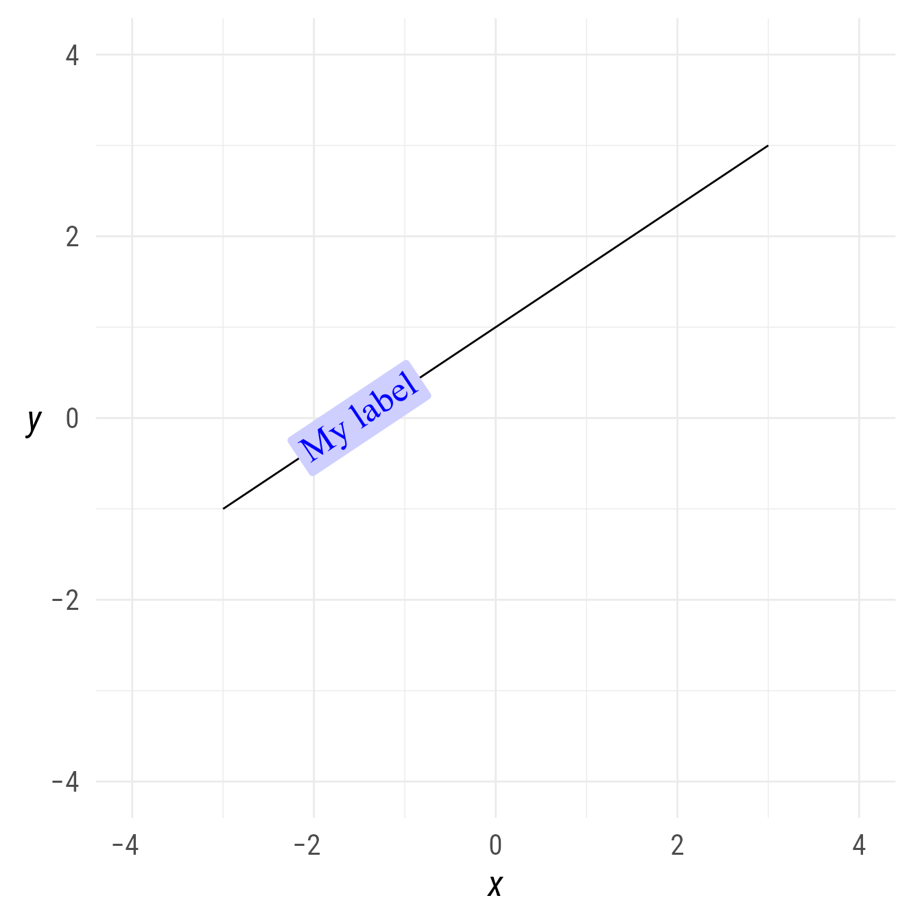
As shown Figure 10, the ob_label function gives much more control over how and where the label will appear.

bp + ob_segment(p1, p2, 
                label = ob_label(
                  label = "My label", 
                  position = .25, 
                  color = "blue", 
                  fill = class_color("blue")@lighten(), 
                  family = "serif", 
                  label.padding = ggplot2::margin(t = 5,r = 4,b = 3,l = 4)))

Figure 10: Segments with arrowheads and fins