Setup
Packages
Base Plot
To avoid repetitive code, we make a base plot:
#| label: baseplot

my_font <- "Roboto Condensed"
my_font_size <- 20
my_point_size <- 2

# my_colors <- viridis::viridis(2, begin = .25, end = .5)
my_colors <- c("#3B528B", "#21908C")

theme_set(
  theme_minimal(
    base_size = my_font_size,
    base_family = my_font) +
    theme(axis.title.y = element_text(angle = 0, vjust = 0.5)))

bp <- ggdiagram(
  font_family = my_font,
  font_size = my_font_size,
  point_size = my_point_size,
  linewidth = .5,
  theme_function = theme_minimal,
  axis.title.x =  element_text(face = "italic"),
  axis.title.y = element_text(
    face = "italic",
    angle = 0,
    hjust = .5,
    vjust = .5)) +
  scale_x_continuous(labels = signs_centered,
                     limits = c(-4, 4)) +
  scale_y_continuous(labels = signs::signs,
                     limits = c(-4, 4))
Specifying a Circle
Circles can be specified by a point at the circle’s center (x0, y0) and a radius r (the distance from the center to the circle’s edge).
Code
bp +
  c1 +
  ob_segment(
    c1@center,
    c1@point_at(0),
    color = my_colors[1],
    label = ob_label(paste0("*r* = ", c1@radius), angle = 0, vjust = 0)
  ) +
c1@center@label(vjust = 1.2, plot_point = TRUE) 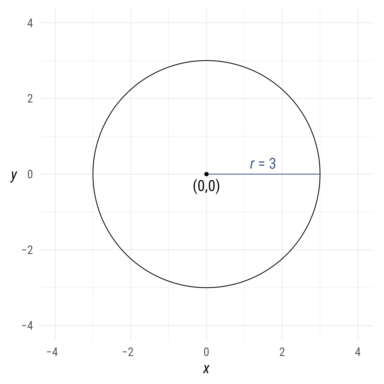
Point on the circle at a specific angle
It is common to need one or more points at a specific angle.
c1@point_at(degree(60))
#>
#> ── <ob_polar>
#> # A tibble: 1 × 2
#>       x     y
#>   <dbl> <dbl>
#> 1   1.5  2.60
Code
deg <- degree(60)

bp +
  c1 +
  {p45 <- c1@point_at(deg)} +
  p45@label(polar_just = ob_polar(deg, 1.5)) +
  ob_segment(c1@center, p45) +
  ob_arc(radius = 1, start = degree(0), end = deg, label = deg)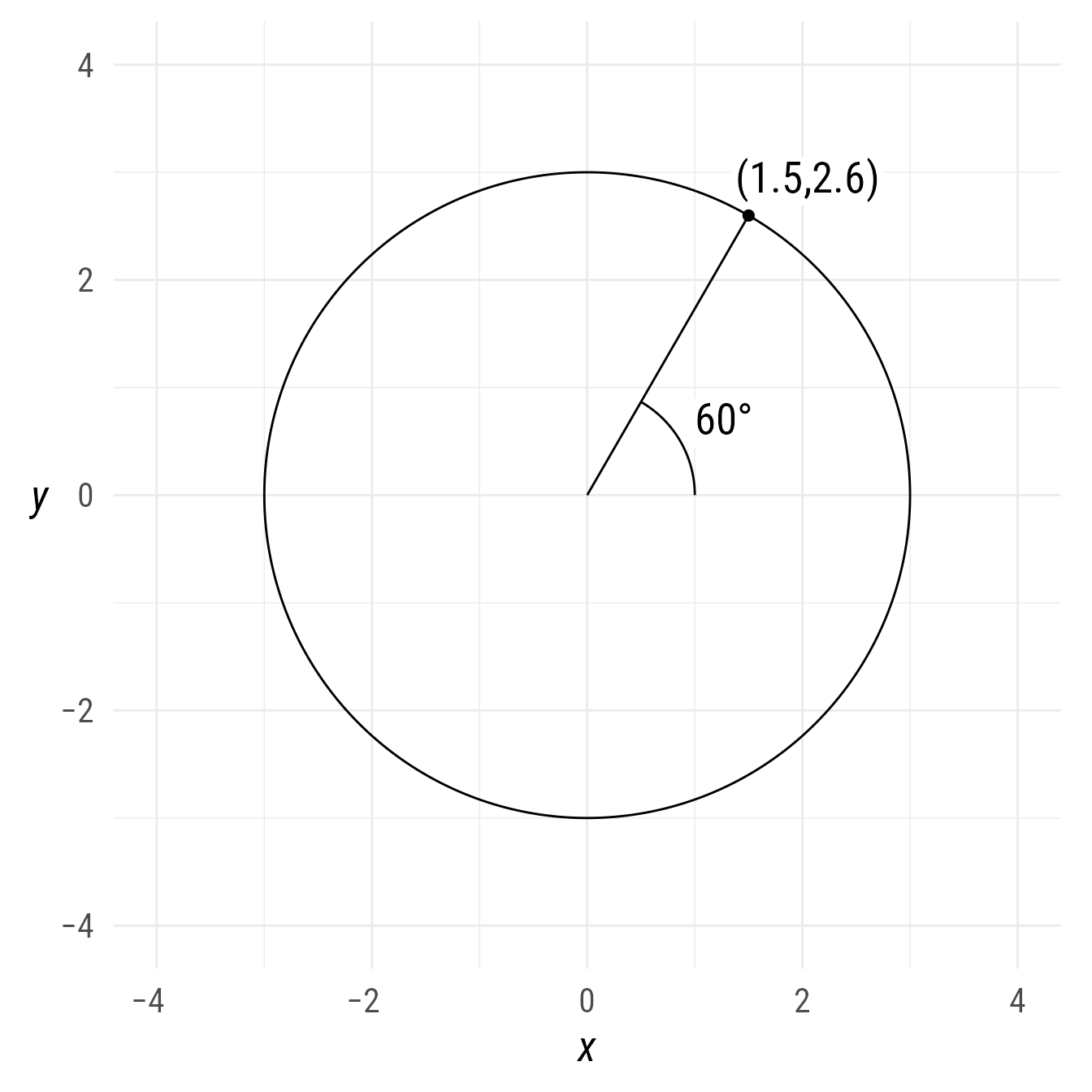
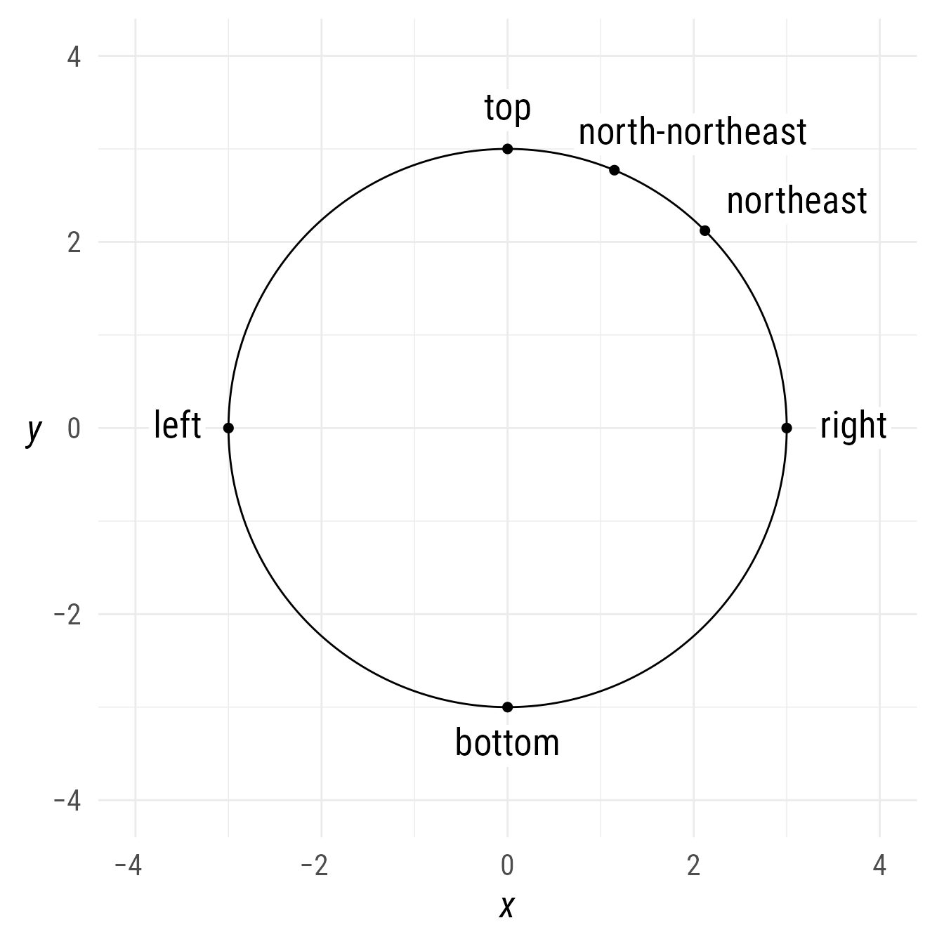
Multiple points can be specified at once.
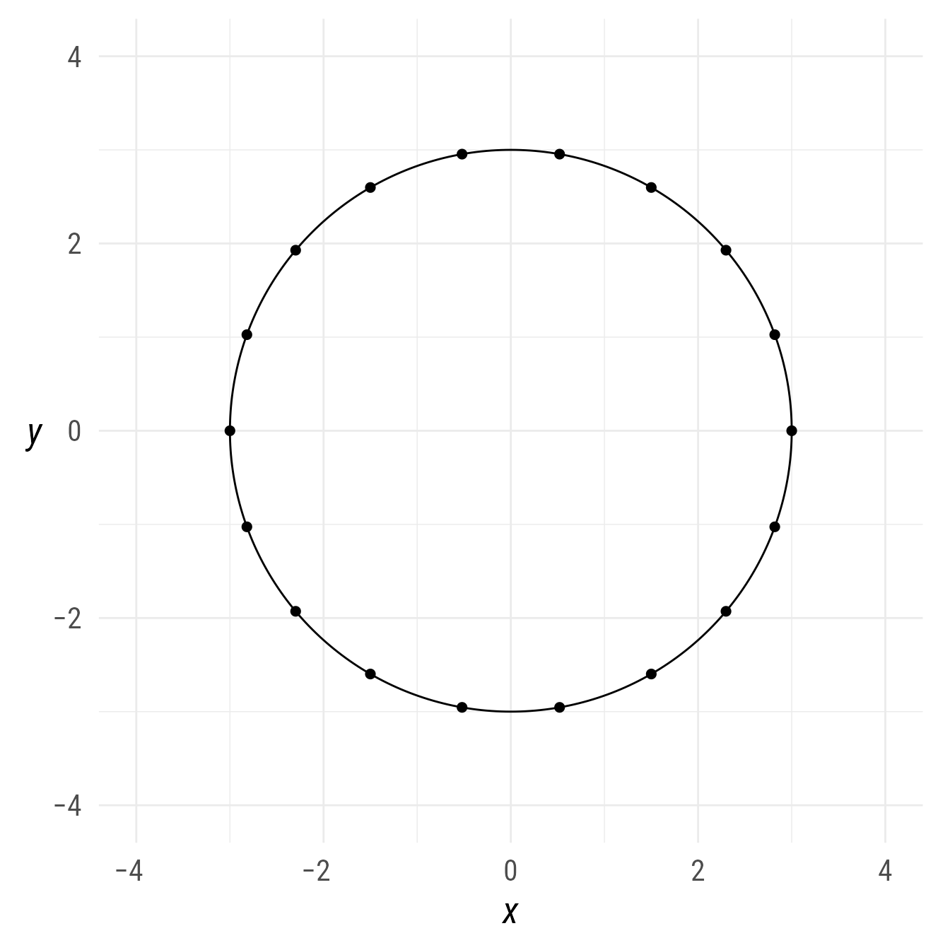
These can be named points (e.g., north|top|above, south|bottom|below, east|right, west|left, northwest|top left|above left, southeast|bottom right|below right, north-northwest).
Placing circles
Placing circles next to each other
The place function places an object at a specified direction and distance from another object.
bp +
  {A <- ob_circle(
    center = ob_point(-2, 0),
    radius = 1,
    label = ob_label("A", size = 30))} +
  place(
    ob_circle(radius = 1.5,
           label = ob_label("B", size = 30)),
    from = A,
    where = "right",
    sep = 1)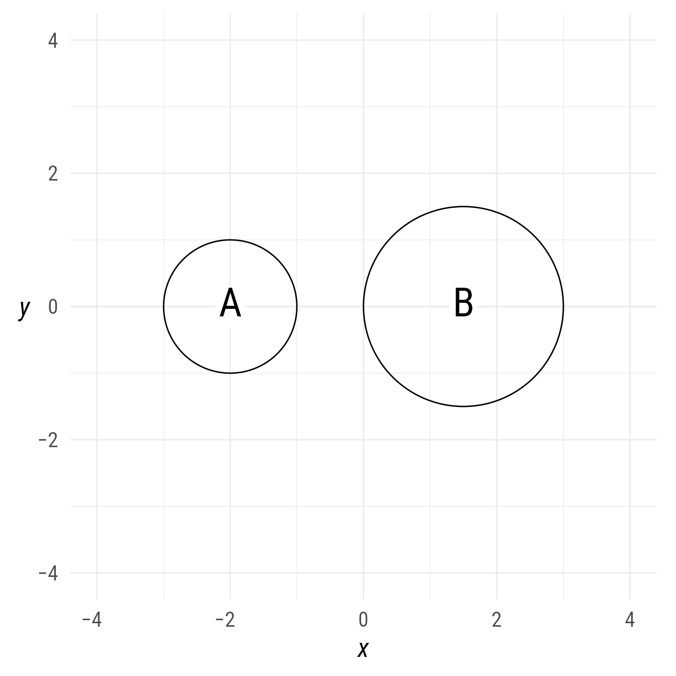
The where argument can take degrees or named positions:
east, right, east-northeast, northeast, top right, above right, north-northeast, north, top, above, north-northwest, northwest, top left, above left, west-northwest, west, left, west-southwest, southwest, bottom left, below left, south-southwest, south, bottom, below, south-southeast, southeast, bottom right, below right, east-southeast
Multiple circles can be created at once with named directions:
bp +
  {c3 <- ob_circle(ob_point(0, 0), radius = 1)} +
  place(ob_circle(radius = .5),
        from = c3,
        where = c("northwest",
                  "northeast",
                  "south-southeast",
                  "south-southwest"),
        sep = 1)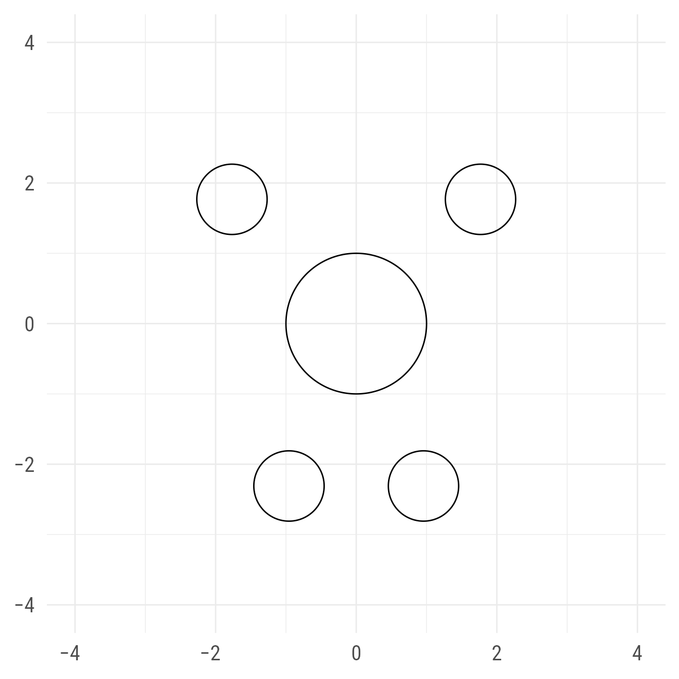
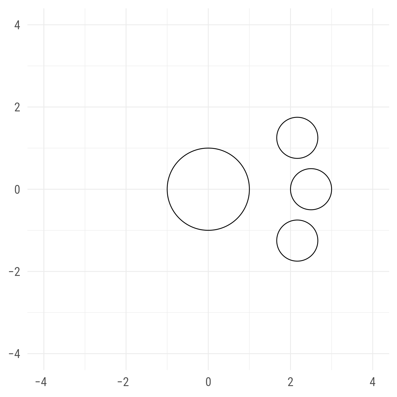
Or with numbers (degrees):
With styles:
Placing circles next to points and points next to circles
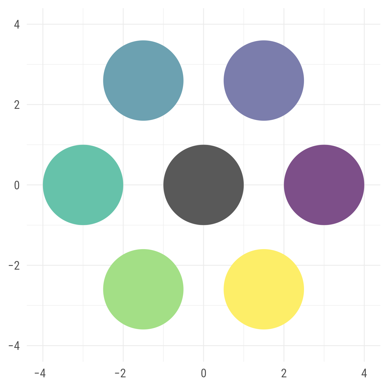
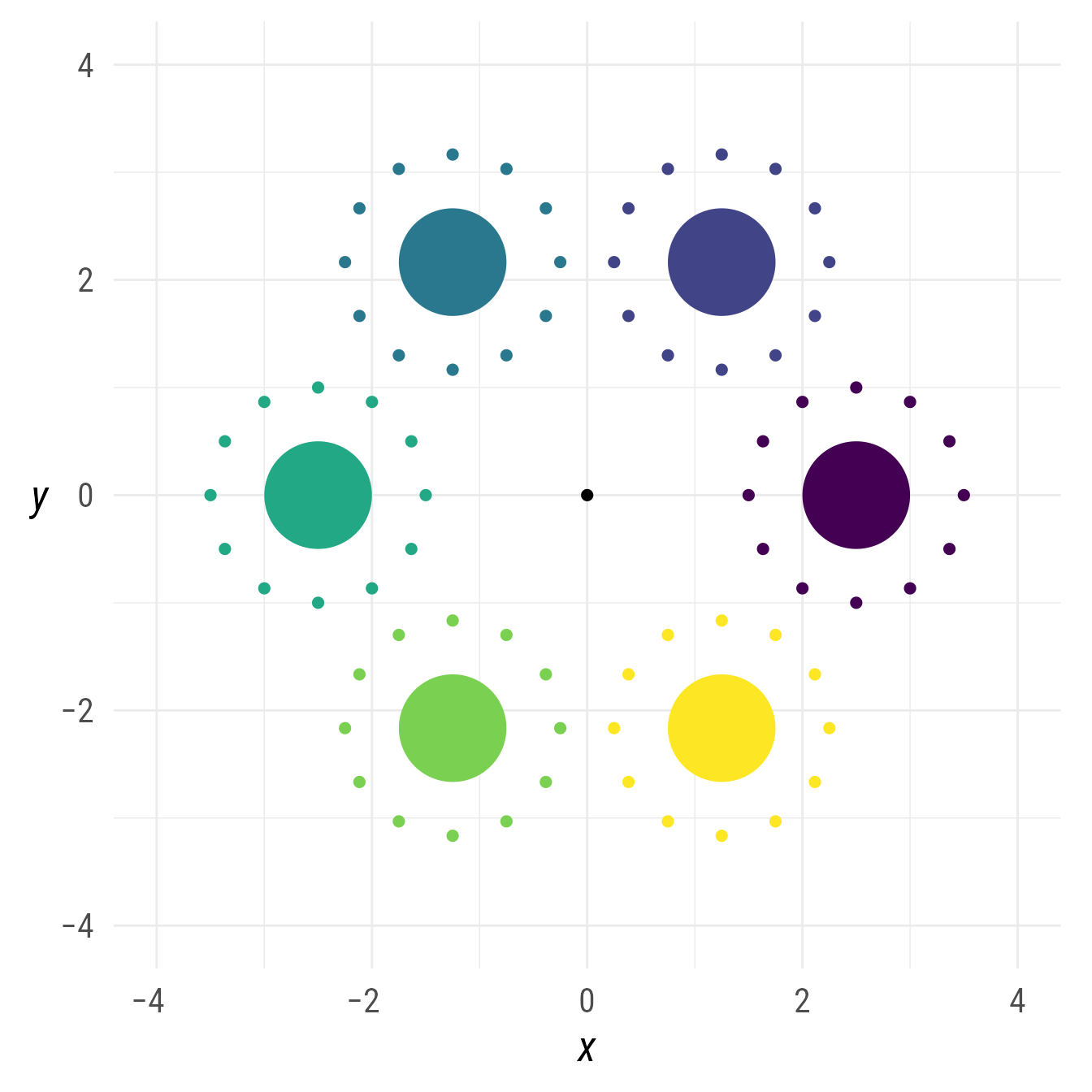
This works the same as placing circles next to each other. Here we create a point in the center, place six circles around it, and then place 12 points around each circle using the map_ob function to “map” objects like the map_* functions in the purrr package.
bp +
  {p1 <- ob_point(0, 0)} +
  {c6 <- place(
      x = ob_circle(
        radius = .5,
        fill = viridis::viridis(6),
        color = NA
      ),
      from = p1,
      where = degree(seq(0, 300, 60)),
      sep = 2
    )} +
  map_ob(unbind(c6),
         \(x) ob_point(color = x@fill) |>
           place(
             from = x,
             where = degree(seq(0, 330, 30)),
             sep = .5
           ))
Placing lines next to circles
Drawing path connectors between circles
Let’s make two circles and draw an arrow path between them
bp +
  {c1 <- ob_circle(ob_point(-2, 2), radius = 1)} +
  {c2 <- ob_circle(ob_point(1.5,-1.5), radius = 1.5)} +
  connect(c1, c2)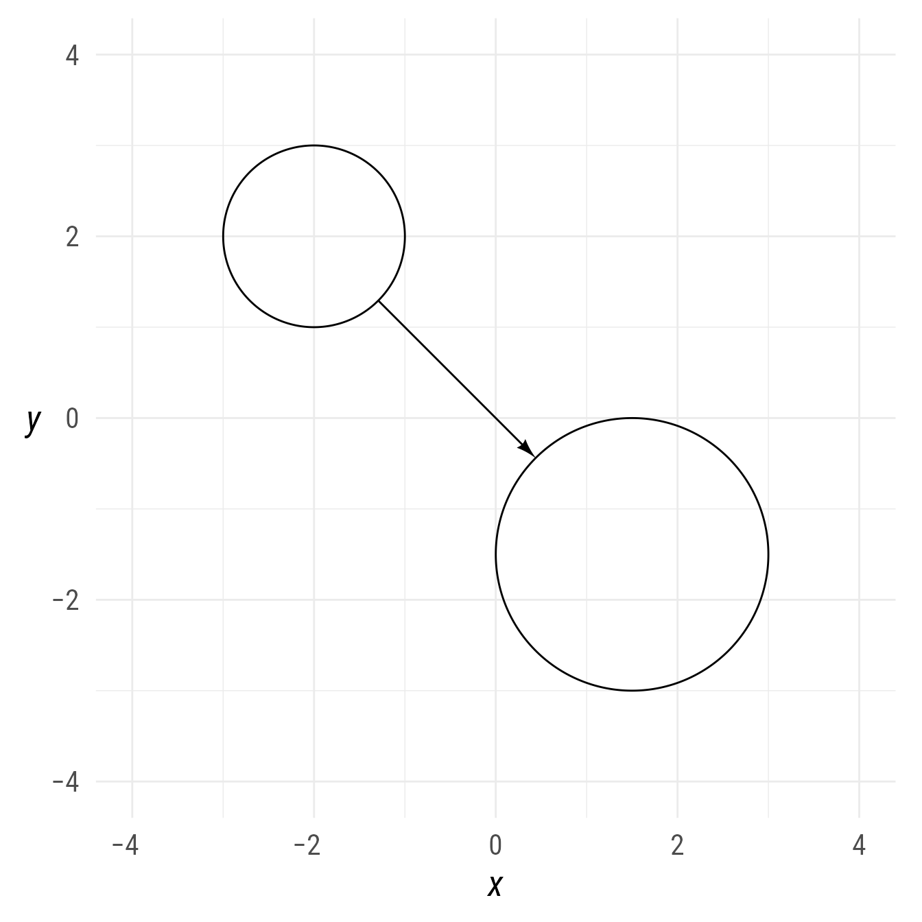
That is fine, but we often need labels and styling to make scientific diagrams. For example:
bp +
  {cthis <- ob_circle(
    ob_point(-2, 2),
    radius = 1,
    fill = my_colors[1],
    color = NA,
    label = ob_label(
      "This",
      color = "white",
      fill = NA,
      size = 35
    )
  )} +
  {cthat <- ob_circle(
    ob_point(1.5, -1.5),
    radius = 1.5,
    fill = my_colors[2],
    color = NA,
    label = ob_label(
      "That",
      color = "white",
      fill = NA,
      size = 55
    )
  )} +
  connect(cthis, cthat,
       resect = 2,
       label = ob_label("Causes", size = 20, vjust = 0),
       color = "black")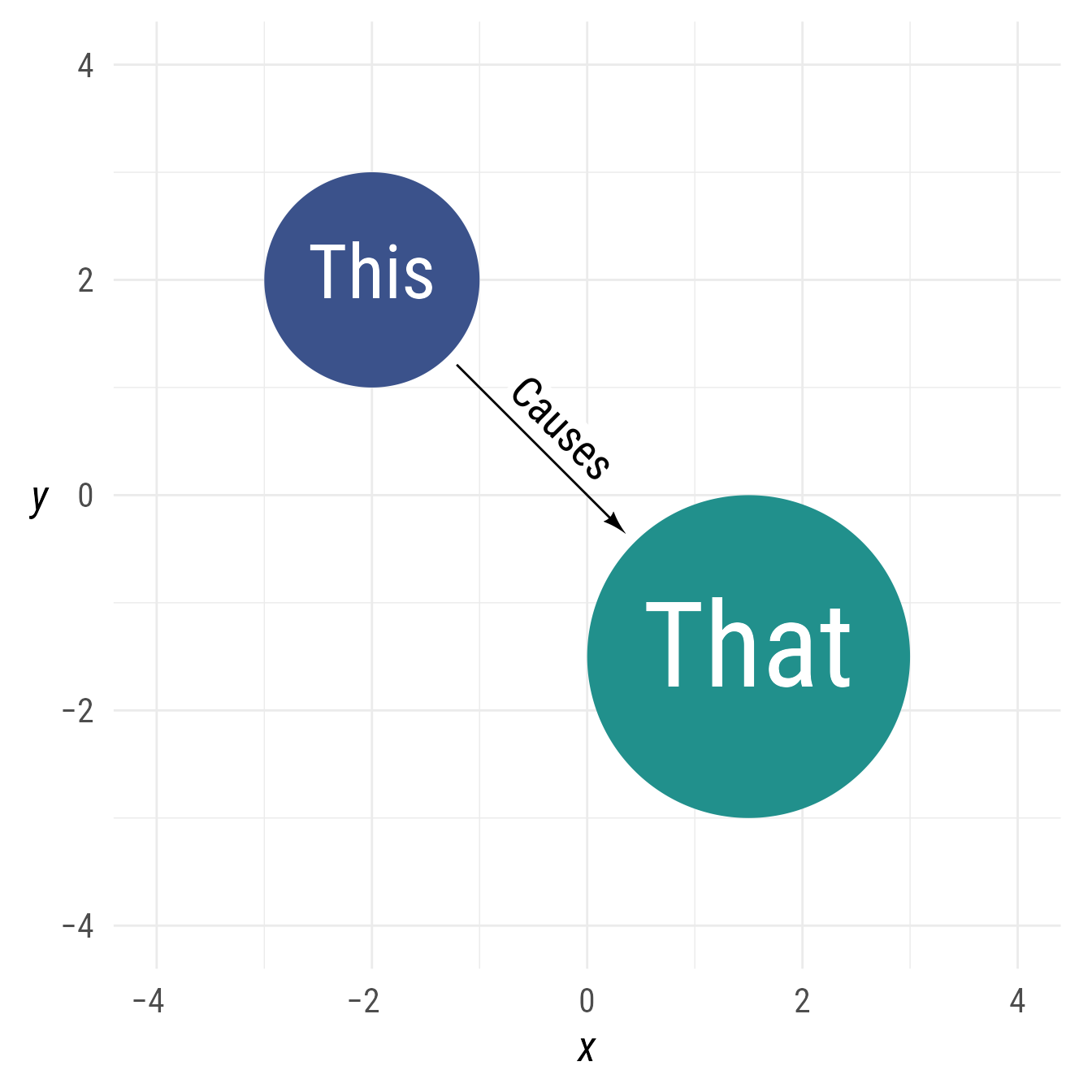
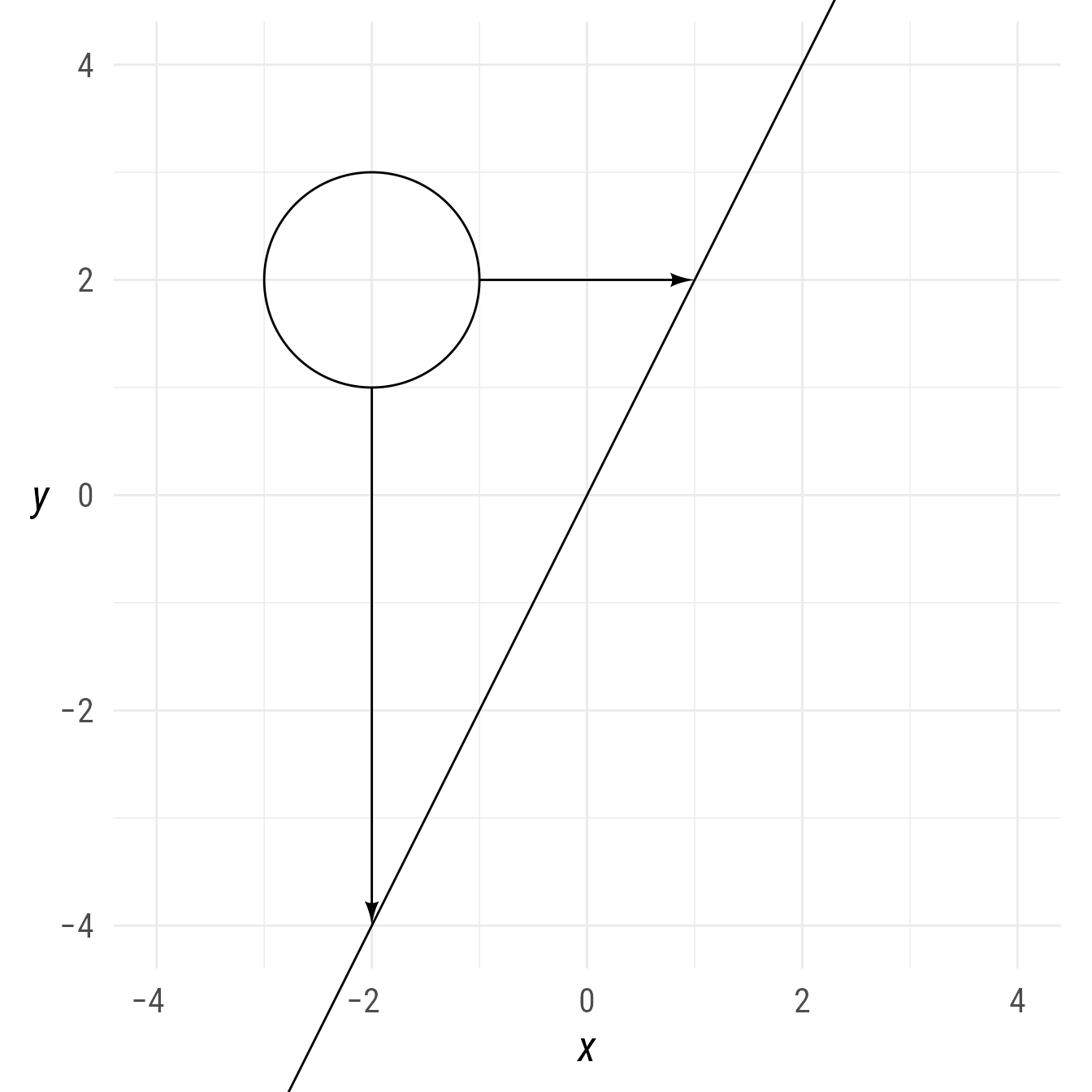
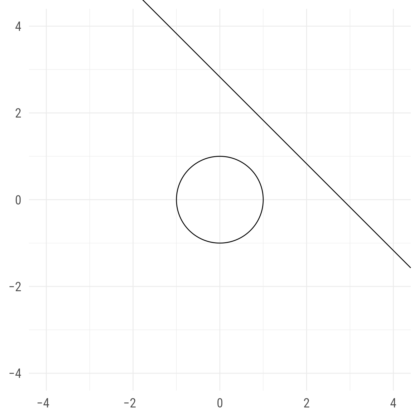
Paths between circles and lines
To connect a circle and the shortest distance to a line:
bp +
  c1 +
  {l1 <- ob_line(slope = 2, intercept = 0)} +
  connect(c1, l1) +
  {c2 <- ob_circle(ob_point(2, -2))} +
  connect(l1, c2)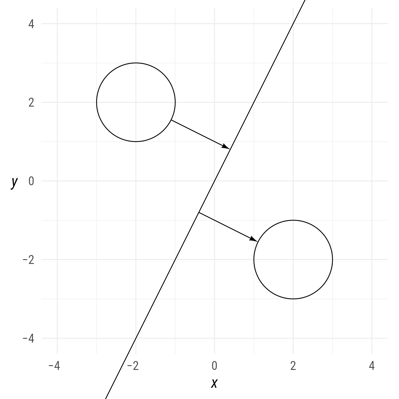
To connect a circle to some other point on the line, we can use the the @point_at_x or @point_at_y function from the ob_line object. For example, to connect from a circle to a line horizontally and vertically: