Setup
Packages
Base Plot
To avoid repetitive code, we make a base plot:
my_font <- "Roboto Condensed"
my_font_size <- 20
my_point_size <- 2

# my_colors <- viridis::viridis(2, begin = .25, end = .5)
my_colors <- c("#3B528B", "#21908C")

bp <- ggdiagram(
  font_family = my_font,
  font_size = my_font_size,
  point_size = my_point_size,
  linewidth = .5,
  theme_function = theme_minimal,
  axis.title.x =  element_text(face = "italic"),
  axis.title.y = element_text(
    face = "italic",
    angle = 0,
    hjust = .5,
    vjust = .5)) +
  scale_x_continuous(labels = signs_centered,
                     limits = c(-4, 4)) +
  scale_y_continuous(labels = signs::signs,
                     limits = c(-4, 4))
Arcs
Just as a segment is part of a line between two points on the line, an arc is part of a circle between two points (on the circle). Thus, an arc has all the properties a circle, with the addition of starting and ending points. For the sake of simplicity, these starting points are specified as angles.
Arc starting and ending points can be specified with any angle unit (e.g., degree(180), radian(pi), turn(0.5)). If a number is used, it will be interpreted as a degree unit.
Code
bp +
  {p1 <- ob_point(0, 0)} +
  {a1 <- ob_arc(
    center = p1,
    radius = {r <- 4},
    start = {ang_start <- degree(25)},
    end = {ang_end <- degree(75)}
    )} +
  ob_label(
    label = paste0("Center ", p1@auto_label),
    center = p1,
    vjust = 1.1) +
  connect(
    p1,
    a1@midpoint(),
    label = paste0("Radius = ", r)) +
  ob_label(
    label = ang_start,
    center = a1@midpoint(0),
    polar_just = ob_polar(ang_start + degree(-90), 1.3),
    plot_point = TRUE) +
  ob_label(
    label = ang_end,
    center = a1@midpoint(1),
    polar_just = ob_polar(ang_end + degree(90), 1),
    plot_point = TRUE)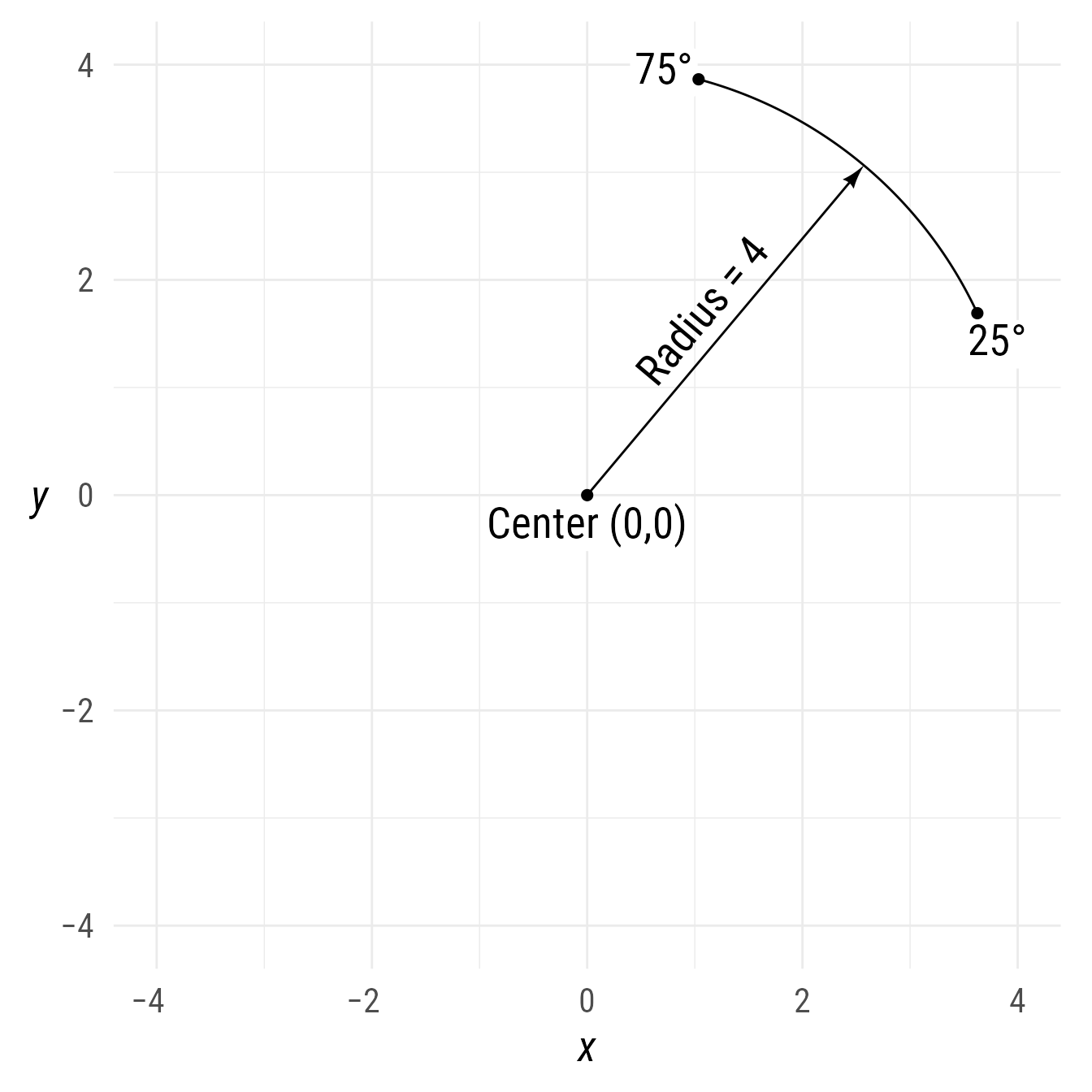
Starting or ending points of arcs
Sometimes you do not know where the center of an arc should be. Instead, you want the arc to start or end at a specific point. For example, you might want to specify the start point or the end point.
p1 <- ob_point(0, 0)

bp +
    ob_arc(start = -45,
      end = 45,
      radius = 2,
      color = "orchid4",
      start_point = p1)  +
  ob_arc(start = -45,
      end = 45,
      radius = 2,
      color = "forestgreen",
      end_point = p1) +
p1 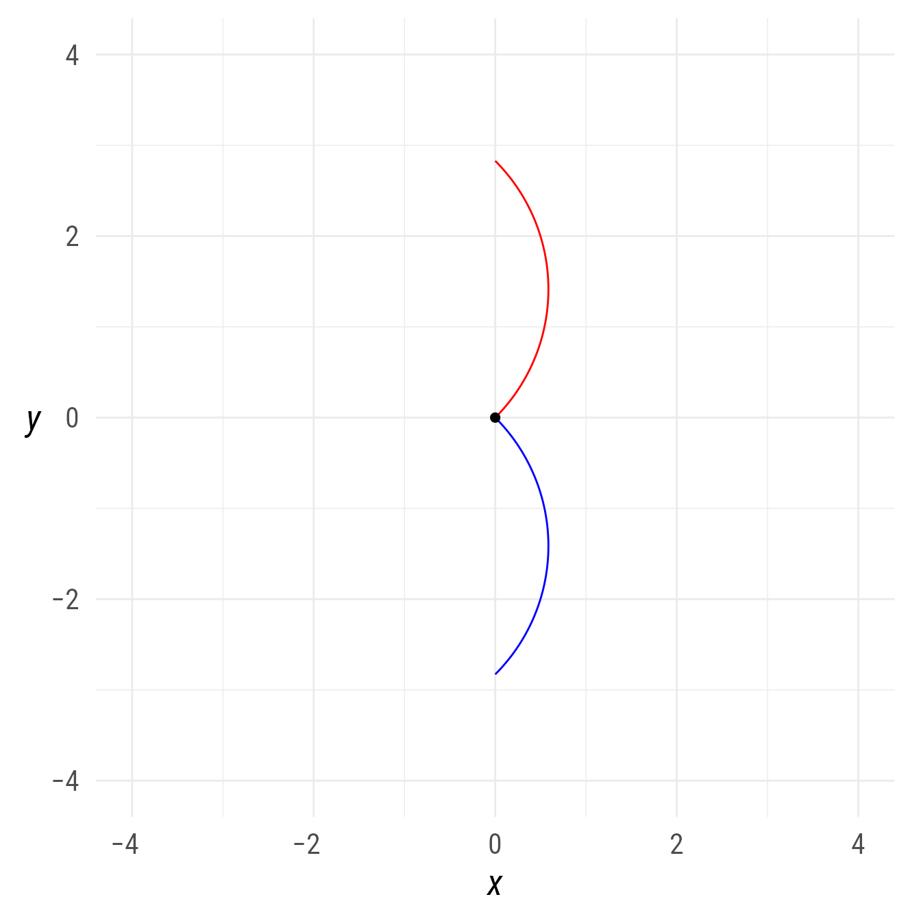
As a example, I used the start_point argument to recreate a fun meme about a “square” object with 4 equal sides that meet at right angles:
little_r <- 1 / (2 * pi - 1)
ggdiagram(font_family = my_font,
          font_size = my_font_size) +
  {p1 <- ob_point(0,0)} +
  {p2 <- ob_point(1,0)} +
  ob_segment(p1, p2) +
  {a1 <- ob_arc(
    start = 0,
    end = radian(1),
    radius = 1 + little_r,
    start_point = p2)} +
  {p3 <- a1@midpoint(1)} +
  {p4 <- a1@normal_at(radian(1),
                      distance = -1)} +
  ob_segment(p3, p4) +
  ob_arc(start_point = p4,
         radius = little_r,
         start = radian(1),
         end = turn(1))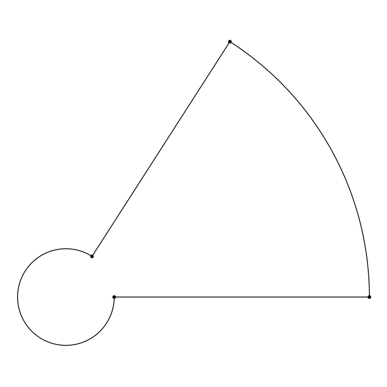
Midpoints
The midpoint function can find one or more midpoints at different positions. The default position is .5.
bp +
  a1 +
  a1@midpoint()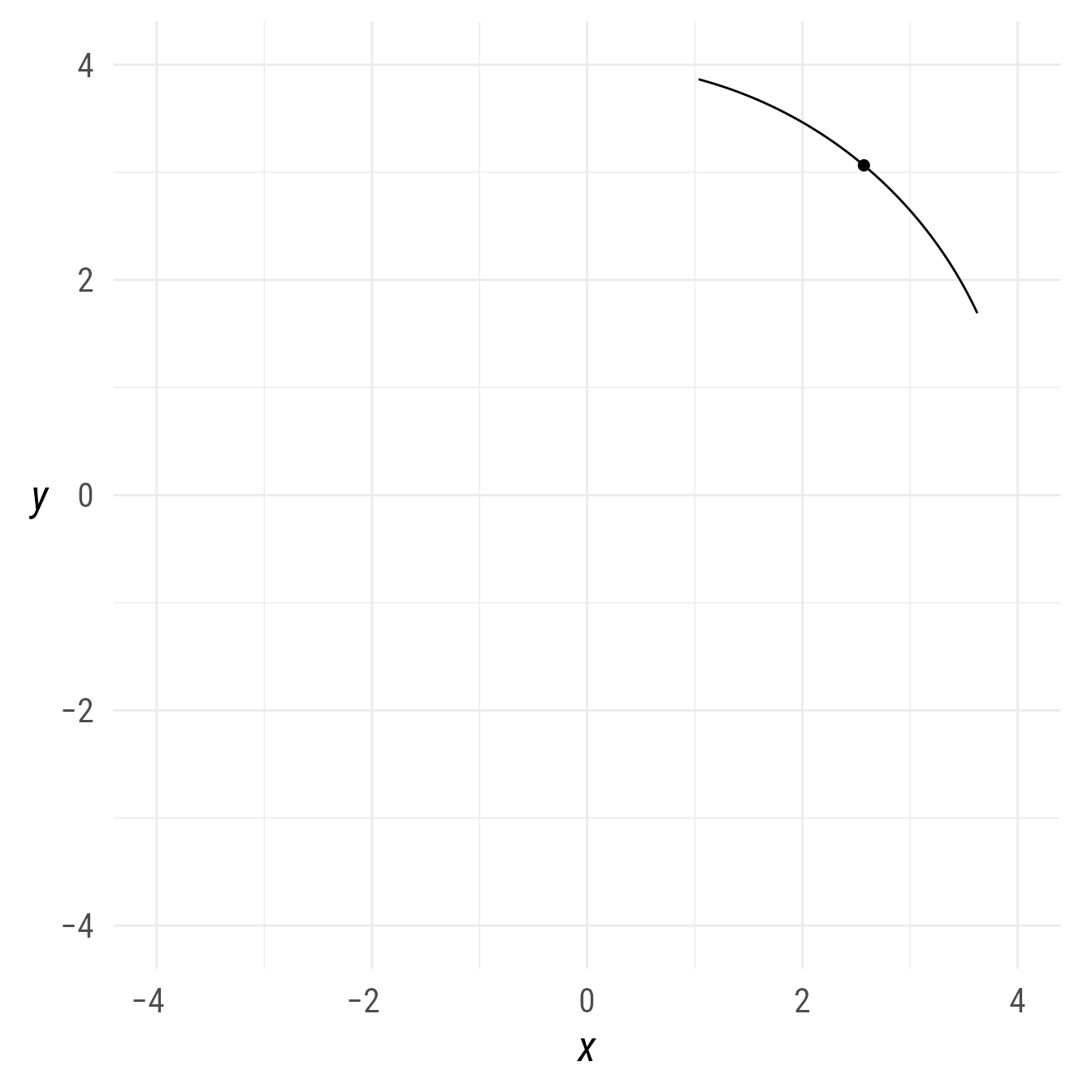
The starting and ending points are at position 0 and 1, respectively.
bp +
  a1 +
  a1@midpoint(position = c(0,1))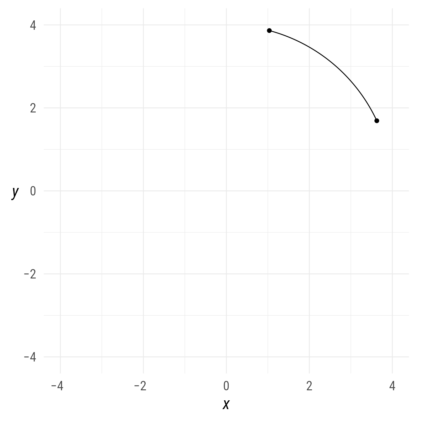
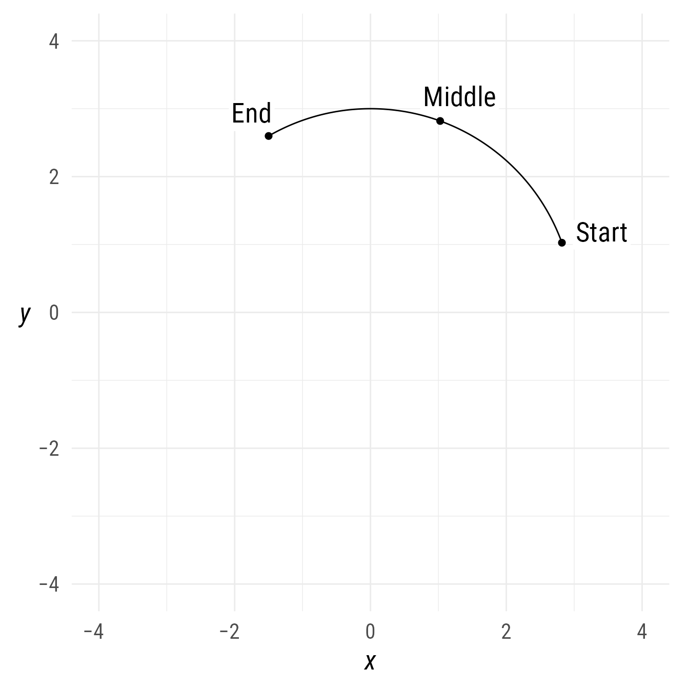
Labelling arcs
By default, the arc label will appear outside the midpoint of the arc

If a label is needed elsewhere, it can be set with the label function’s position property.
bp +
  ob_arc(
    radius = 3,
    start = 20,
    end = 120,
    label = ob_label(
      c("Start", "Middle", "End"),
      position = c(0, .5, 1),
      plot_point = TRUE
    )
  )
If the orientation of the label needs to be changed, it can be set with vjust, hjust, or polar_just.
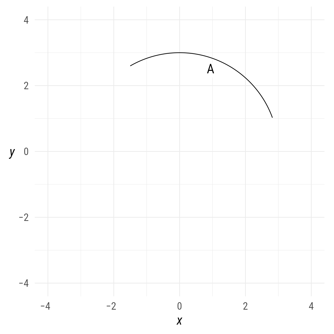
There are cases where the arc is already created and a label is needed. Although the label can be added after the arc has been created, the position would have to be set manually (otherwise the position will be at 0,0 by default). In such cases, the auto_label function can help place the label correctly. By default, the auto_label will show the the theta property (i.e., end − start).
bp +
  {a1 <- ob_arc(radius = 3,
      start = 20,
      end = 120)} +
  a1@auto_label()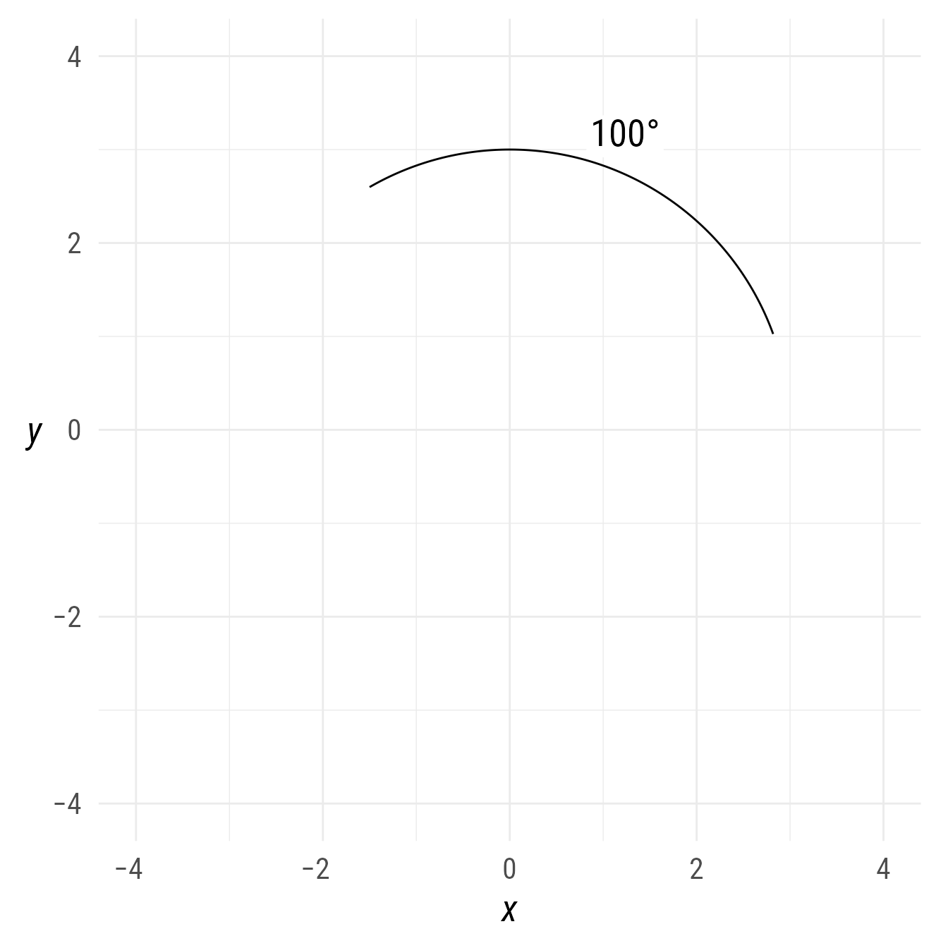
However, any label can be inserted at any position.
bp +
  a1 +
  a1@auto_label(label = "Start",
               position = 0)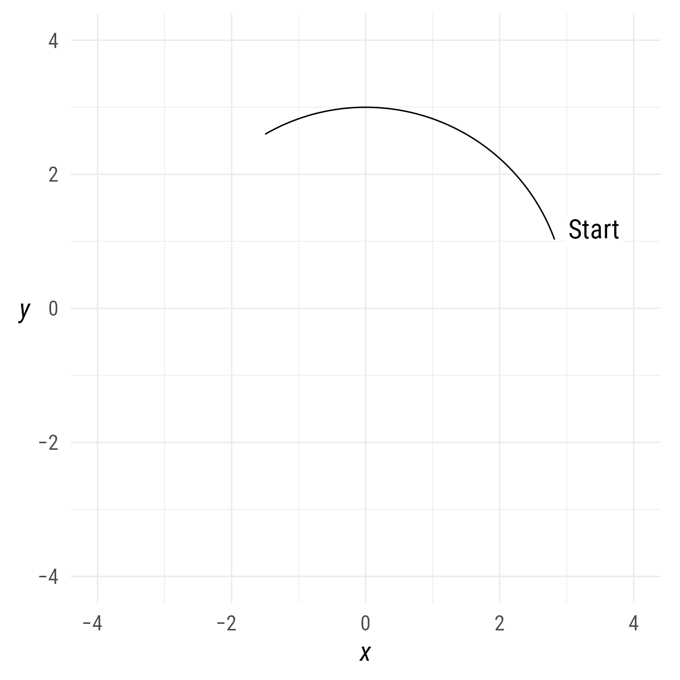
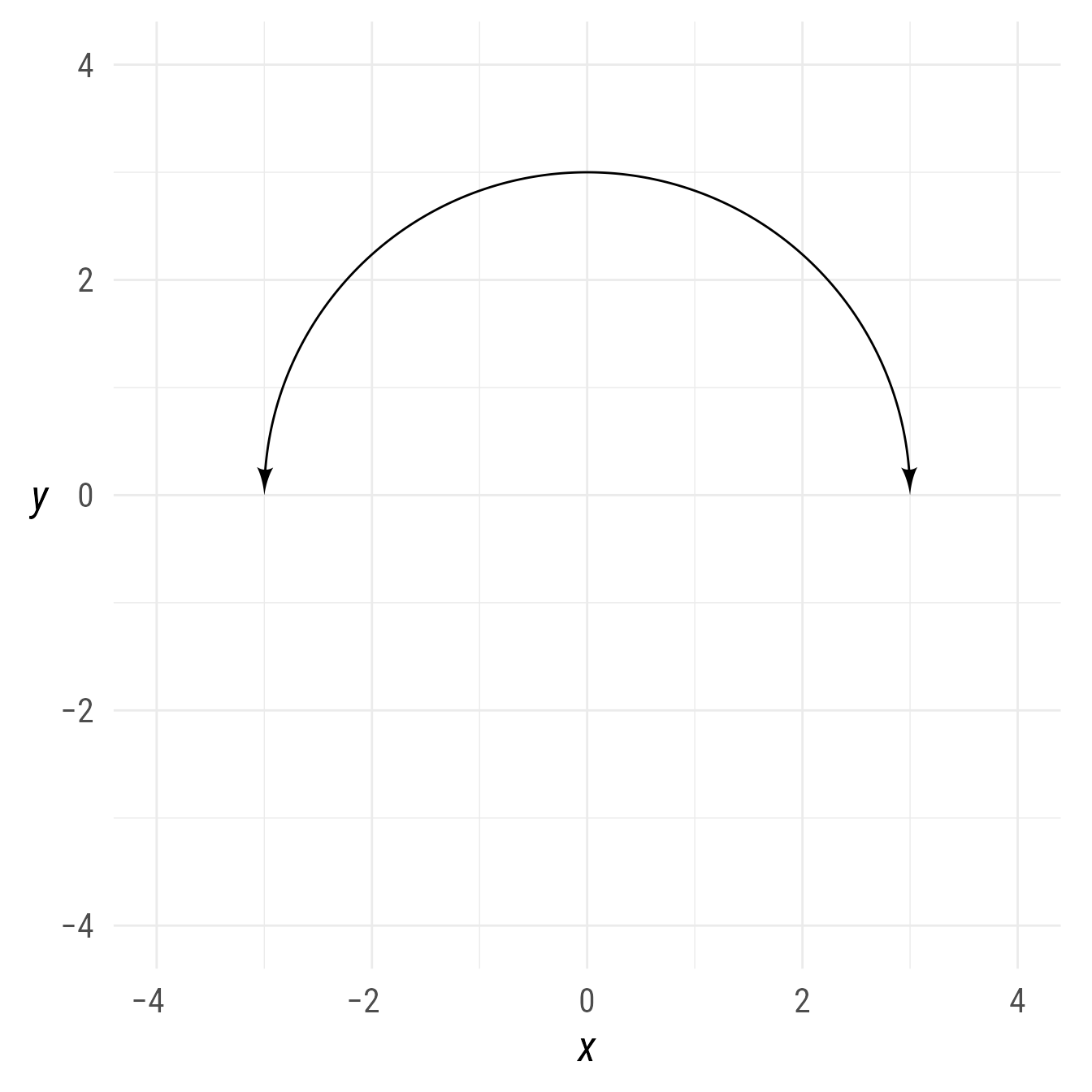
Arcs with arrows
The arc object is plotted using ggarrow::arrow. This means that arrows can be placed on either end of an arc.
Connecting Points and Shapes with Arcs
The connect function makes it easy to draw connectors between points and/or shapes. Normally the connector is a line segment but it is possible to connect with arcs and bezier curves. To connect two shapes with an arc, set the arc_bend parameter.
Negative values bend left, and positive values bend right. By default, a value of 1 or -1 makes a full semi-circular path between the centers of the shapes. Values close to 0 make the arc appear more straight. Large values make the circle the arc follows larger. The arc_bend specifically refers to ratio of arc’s sagitta to the arc’s radius. Thus, arc_bend cannot actually be set to 0, because this would cause an infinite ratio.
By default, the connector is drawn such that the arc would pass through the shape’s center if allowed to continue. If you want the arc to begin or end somewhere else, specify the point. For example, the arc from A to C ends at the bottom of C.
bp +
  {A <- ob_circle(x = -2,
                  label = "A")} +
  {B <- ob_ellipse(x = 1,
                   a = 1,
                   b = .5,
                   angle = degree(60),
                   label = ob_label("B", angle = 0))} +
  {C <- ob_rectangle(center = ob_point(3,0),
                     label = "C")} +
  connect(A, B, arc_bend = -.75) +
  connect(B, C, arc_bend = -1) +
  connect(A, C@south, arc_bend = .6)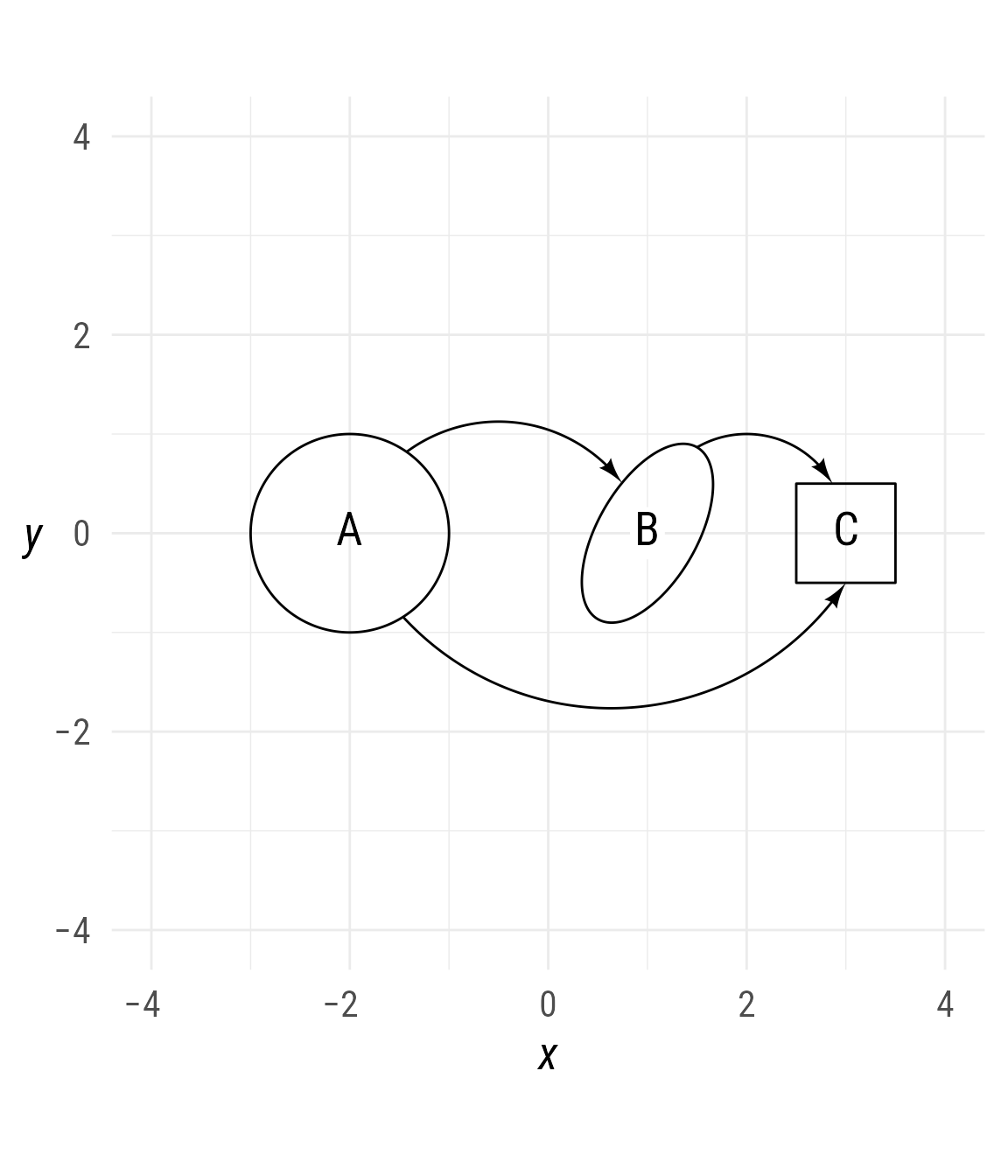
Wedges
The ob_arc function has a @type property that can be set to "arc", "wedge", or "segment". When set to arc, the arc is drawn with geom::arrow so that the arc endpoints can be arrows. Otherwise, when @type is wedge or segment, ob_arc drawn with ggplot2::geom_polygon.
The ob_wedge function is a convenient wrapper function for ob_arc that sets the @type property to wedge.
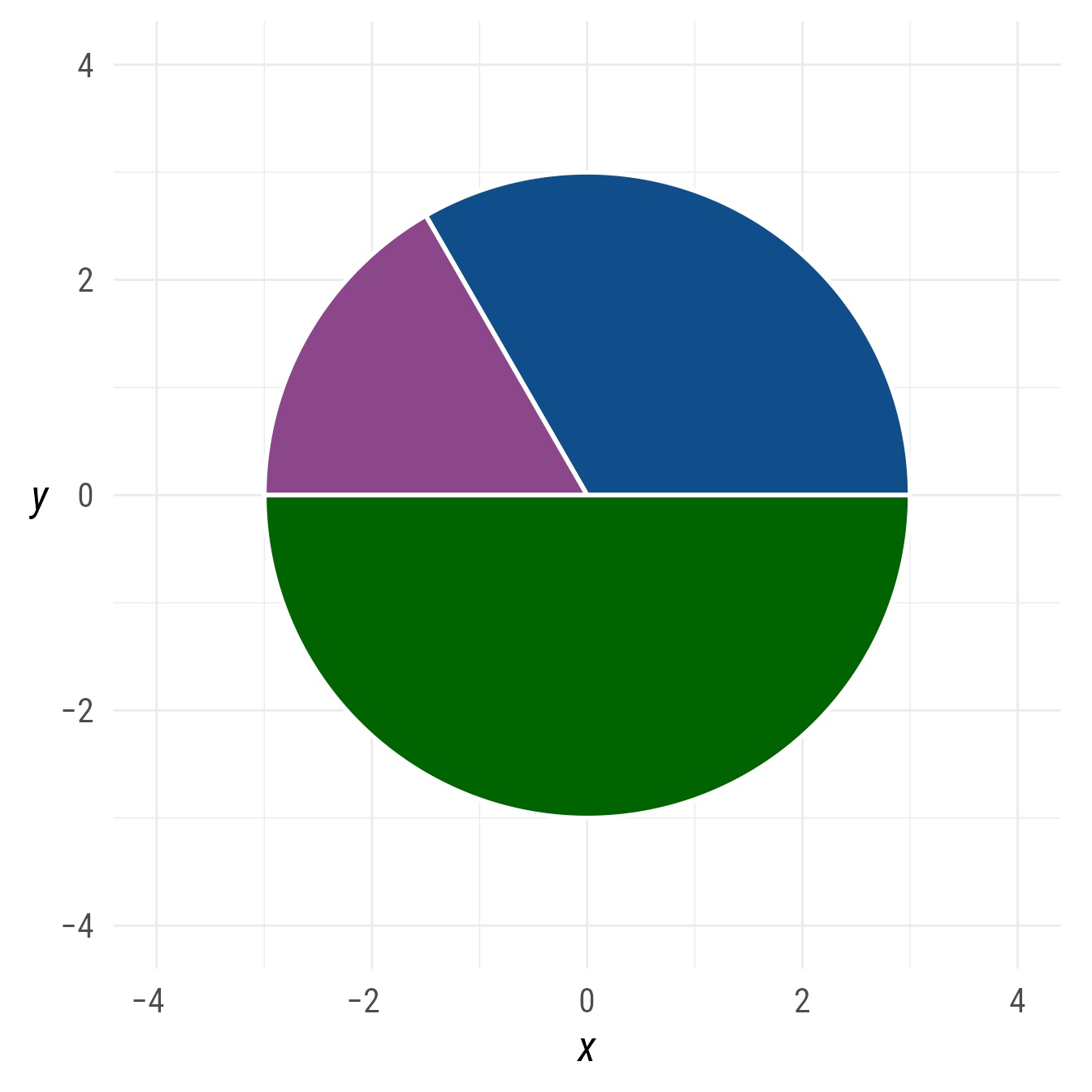
Circular Segments
A circular segment is an arc made into a polygon.
The ob_circular_segment function is a convenient wrapper function for ob_arc that sets the @type property to segment.
theta <- turn(seq(0, 1, 1 / 3) + 1 / 12)

ggdiagram() +
  ob_circular_segment(
    start = theta[-length(theta)],
    end = theta[-1],
    fill = c("dodgerblue4", "orchid4", "darkgreen")
  )
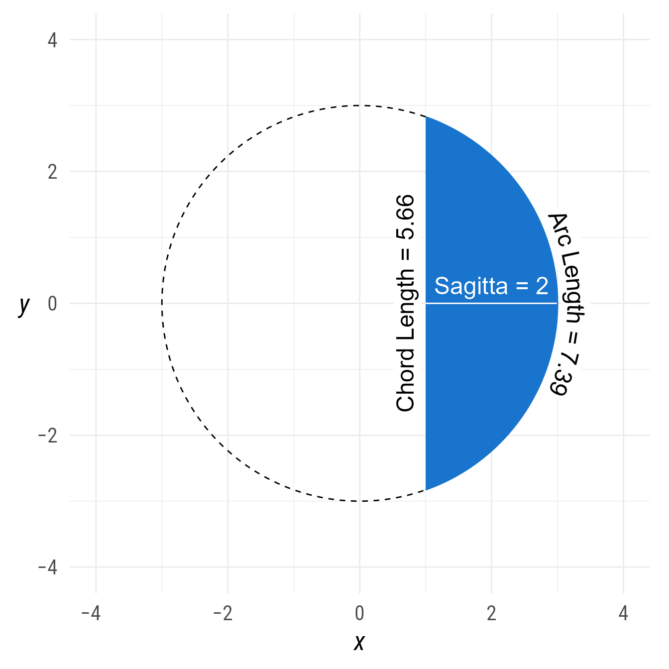
Objects made with ob_arc, ob_wedge, or ob_circular_segment can return important features of arcs, including the chord, sagitta, and arc_length. In Figure 14, the chord is the ob_segment that connects the endpoints of the arc. The sagitta is ob_segment from the arc’s midpoint to the chord’s midpoint. Not shown in Figure 14, the apothem is the ob_segment from the arc’s center point to the midpoint of the chord. The radius is the sum of the distances spanned by the apothem and the sagitta.
bp +
  {cs <- ob_circular_segment(
      radius = 3,
      end = radian(-acos(1 / 3)) + degree(45),
      start = radian(acos(1 / 3)) + degree(45),
      fill = "dodgerblue3",
      label_sloped = TRUE
    )
  cs <- cs %>% set_props(
    label = ob_label(
      paste0("Arc Length = ", round(cs@arc_length, 2)),
      vjust = -0.1,
      size = 18,
      color = "black"))
    } +
  ob_arc(
    radius = 3,
    start = cs@start,
    end = cs@end + degree(360),
    linetype = "dashed"
  ) +
  cs@chord@midpoint()@label(
    paste0("Chord Length = ", round(cs@chord@distance, 2)),
    angle = cs@chord@line@angle ,
    vjust = 1.1,
    color = "black",
    size = 18
  ) +
  cs@sagitta %>% set_props(color = "white", arrow_head = arrowhead()) +
  cs@sagitta@midpoint()@label(
    paste0("Sagitta = ", round(cs@sagitta@distance, 2)),
    vjust = 0,
    angle = cs@sagitta@line@angle,
    size = 18,
    fill = NA,
    color = "white"
  ) +
  connect(cs@center, cs@point_at(degree(225)), color = "black", label = ob_label("Radius = 3", angle = degree(45), size = 18, vjust = 0))
Fun fact: Our geometric concepts arc, chord, and sagitta are all archery terms, deriving from the Latin words arcus (bow), chorda (string), and sagitta (arrow).