Setup
Path diagrams
Structural equation models are often displayed with path diagrams. The visual vocabulary of path diagrams is fairly simple. As seen in Figure 1, an observed variable is a square or rectangle, and a latent variable is a circle or ellipse. Often omitted for clarity, means and intercepts are constants that can be depicted with triangles.
Code
ggdiagram(font_family = my_font, font_size = 16) +
  {lv <- ob_circle(label = "Latent<br>Variable")} +
  {r <- ob_rectangle(width = sqrt(pi),
                  height = sqrt(pi),
                  label = "Observed<br>Variable") |>
    place(lv, "right", .5)} +
  {i <- ob_circle(n = 3,
               radius = 1.25,
               label = "Mean/<br>Intercept") |>
place(r, "right", .3) + ob_point(0, -.25)} 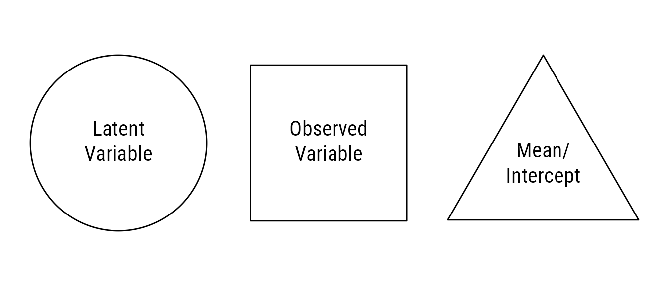
In Figure 2, two types of relationships are depicted. A single-headed arrow indicates a direct causal influence. A curved double-headed arrow indicates a correlation between two variables but does not specify the causal nature of the relationship.
Code
ggdiagram(font_family = my_font, font_size = 16) +
  {this <- ob_circle(label = ob_label("This", size = 40))} +
  {that <- ob_circle(label = ob_label("That", size = 40)) |>
    place(this, "right")} +
  connect(this, that, label = "Causes", resect = 2) +
  {A <- this |>
    place(this, "below")} +
  {B <- that |>
    place(that, "below")} +
ob_covariance(A, B, label = ob_label("Correlates with", vjust = 0), arrowhead_length = 7) 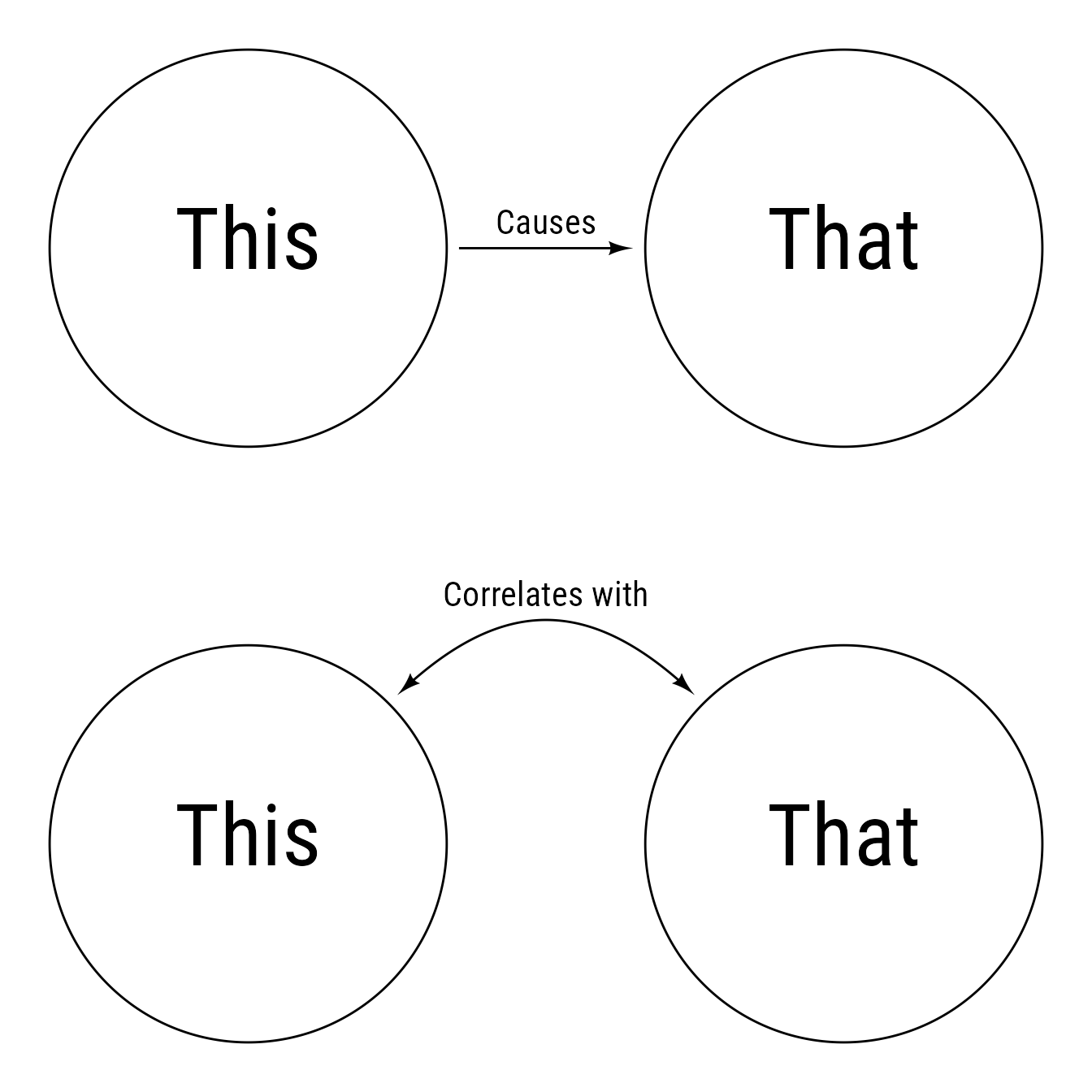
Path Models for Regression
A regression model can be stated very simply: X predicts Y. Most of the time, this relationship can be stated with a simplified path diagram like Figure 3.
Code
observed <- redefault(
  ob_ellipse,
  m1 = 15)
lb_observed <- redefault(
  ob_label,
  size = 48,
  nudge_y = -.15,
  fill = NA)
direct <- redefault(
  connect,
  resect = 2)
lb_direct <- redefault(
  ob_label,
  angle = 0,
  position = .47)

ggdiagram(font_family = my_font, font_size = 16) +
  {X <- observed(label = lb_observed("X"))} +
  {Y <- observed(label = lb_observed("Y")) |>
    place(X,where = "right")} +
  direct(X,Y)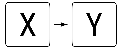
This simple statement skips a large number of details, which can be filled in. The predictor, X is a random variable with an unknown distribution FX. It has a mean of μX and a standard deviation of σX.
Regression takes X and subjects it to a linear transformation to create the variable Ŷ:
The regression coefficients b0 and b1 are known as the intercept and slope, respectively. Ŷ is the predicted value of Y, given X.
The prediction error e is the difference between the actual value of Y and its predicted value Ŷ:
The prediction error is assumed to be normally distributed with a standard deviation of σe, which is known as the standard error of the estimate:
Putting it all together:
All of this can be communicated succinctly with the path diagram in Figure 4.
Code
ln_color <- "gray40"
lb_color <- "gray20"
# Observed variable, label, and variance
observed <- redefault(ob_ellipse,
a = .6,
m1 = 10,
color = ln_color)
lb_observed <- redefault(ob_label,
size = 40,
nudge_y = -.07,
color = lb_color)
var_observed <- redefault(ob_variance,
bend = -25,
looseness = 1.5,
color = ln_color)
# Error variable, label, and variance
error <- redefault(ob_circle, color = ln_color, radius = .5)
lb_error <- redefault(ob_label,
size = 18,
color = lb_color)
var_error <- redefault(ob_variance,
looseness = 1.8,
theta = degree(60),
where = "east",
color = ln_color)
covariance <- redefault(
ob_covariance,
color = ln_color,
bend = 45,
linewidth = .5,
arrowhead_length = 7,
looseness = 1.2
)
# Direct Effect and label
direct <- redefault(connect, resect = 2, color = ln_color)
lb_direct <- redefault(
ob_label,
size = 16,
color = lb_color,
angle = 0,
vjust = .5,
position = .46
)
ggdiagram(font_family = my_font, font_size = 16) +
# Predictor Variable
{X <- observed(label = lb_observed("*X*"))} +
# Predicted Value
{Yhat <- observed(label = lb_observed("*Ŷ*")) |>
place(X, "right", sep = 2)} +
# Outcome Variable
{Y <- observed(
label = lb_observed("*Y*")) |>
place(Yhat, "right", sep = .75)} +
# Error
{e <- error(label = lb_observed("*e*", nudge_y = 0)) |>
place(Y, "right", sep = .75)} +
# Error Variances and labels
{sigma_x <- var_observed(X, where = "west")} +
{sigma_e <- var_error(e, where = "east")} +
ob_latex(tex = c(
r"(\text{\emph{σ}}^{\text{2}}_{\mkern-1.5mu\text{\emph{X}}})",
r"(\text{\emph{σ}}^{\text{2}}_{\mkern-1.5mu\text{\emph{e}}})"),
color = lb_color,
center = bind(c(sigma_x, sigma_e))@midpoint(),
width = .4,
family = my_font) +
# Mean / Intercept
{i <- ob_intercept(
center = ob_polar(theta = degree(60),
distance(X@center,Yhat@center)) +
ob_point(0,-.2),
width = 1.2,
radius = unit(2, "pt"),
fill = NA,
linewidth = .5,
color = ln_color,
label = lb_observed(1, size = 30, nudge_y = 0))} +
# Direct paths
direct(X, Yhat, label = lb_direct("*b*~1~")) +
direct(i, X, label = lb_direct("*μ~X~*")) +
direct(i, Yhat, label = lb_direct("*b*~0~")) +
direct(Yhat,Y) +
direct(e, Y)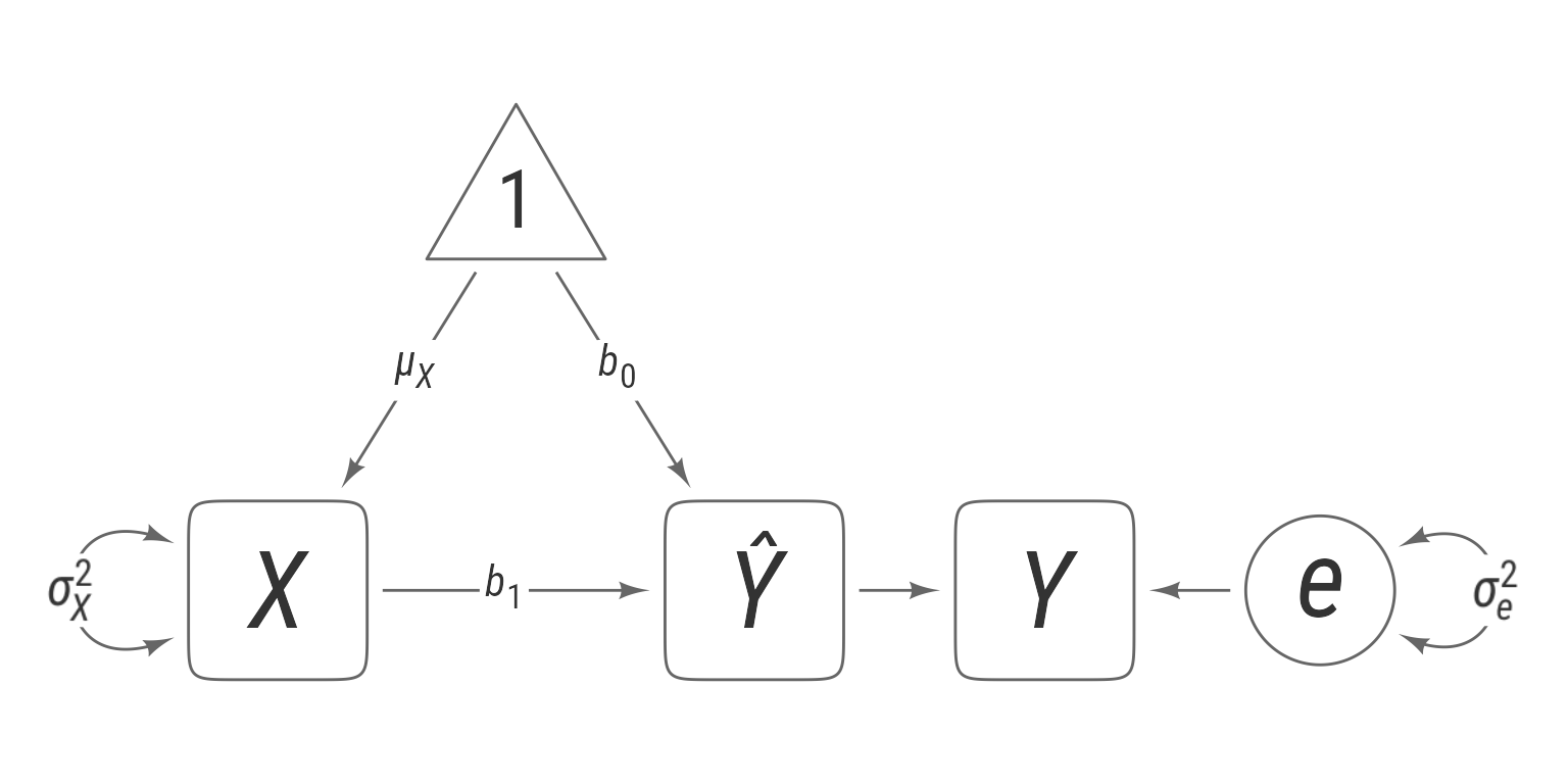
Path Diagrams for Path Analysis
Path diagrams were created by Sewall Wright (1920) to display path analyses—interconnected regression models with sequences of direct and indirect relationships among variables.
For example, these two regression equations combined make up a causal system that shows how variables X1–X4 interrelate.
Code
ggdiagram(font_family = my_font, font_size = 16) +
  {x1 <- observed()
   x2 <- observed() |>
    place(x1, "below", sep = 2.25)
   x3 <- observed() |>
    place(midpoint(x1@east,
                   x2@east),
          "right")
   x4 <- observed() |>
    place(x3, "right", sep = 1.5)
   x <- bind(c(x1, x2, x3, x4))} +
  lb_observed(paste0("*X*~",1:4,"~"), x@center) +
  {pred <-    bind(c(x2, x1, x3, x1, x2))
   outcome <- bind(c(x3, x3, x4, x4, x4))
   direct(pred,outcome,
          label = lb_direct(
            label = c("*b*~23~",
                      "*b*~13~",
                      "*b*~34~",
                      "*b*~14~",
                      "*b*~24~")))} +
  {endogenous <- bind(c(x3,x4))
   e <- error(label = lb_error(paste0("*e*~", 3:4, "~"))) |>
    place(from = endogenous,
          where = c("left", "right"),
          sep = .5)} +
  direct(e, endogenous) +
  covariance(x2@west,
             x1@west,
             label = lb_direct("*r*~12~", position = .5))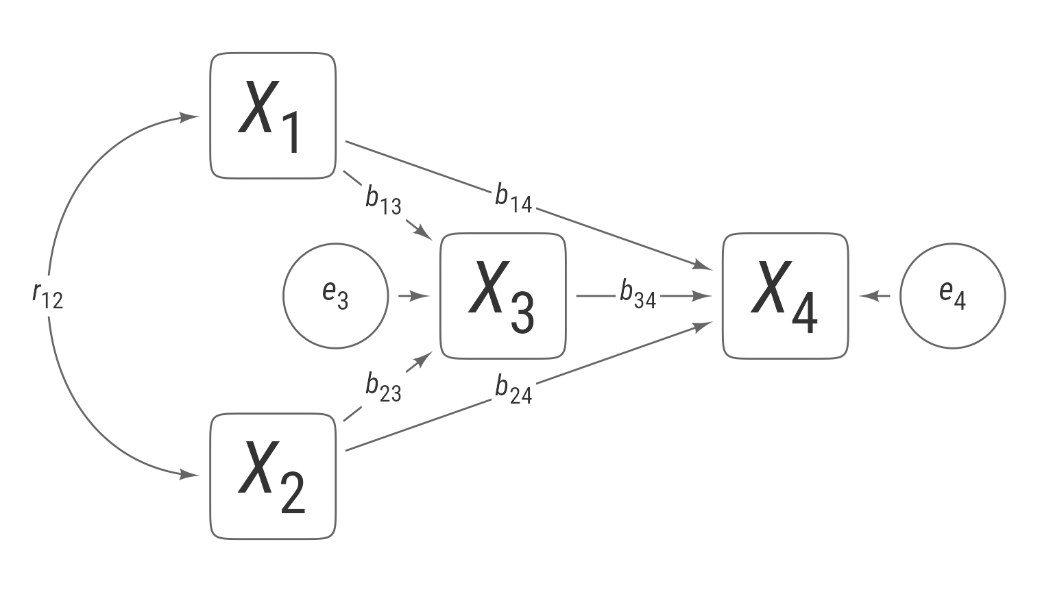
Path Diagrams for Exploratory Factor Analysis
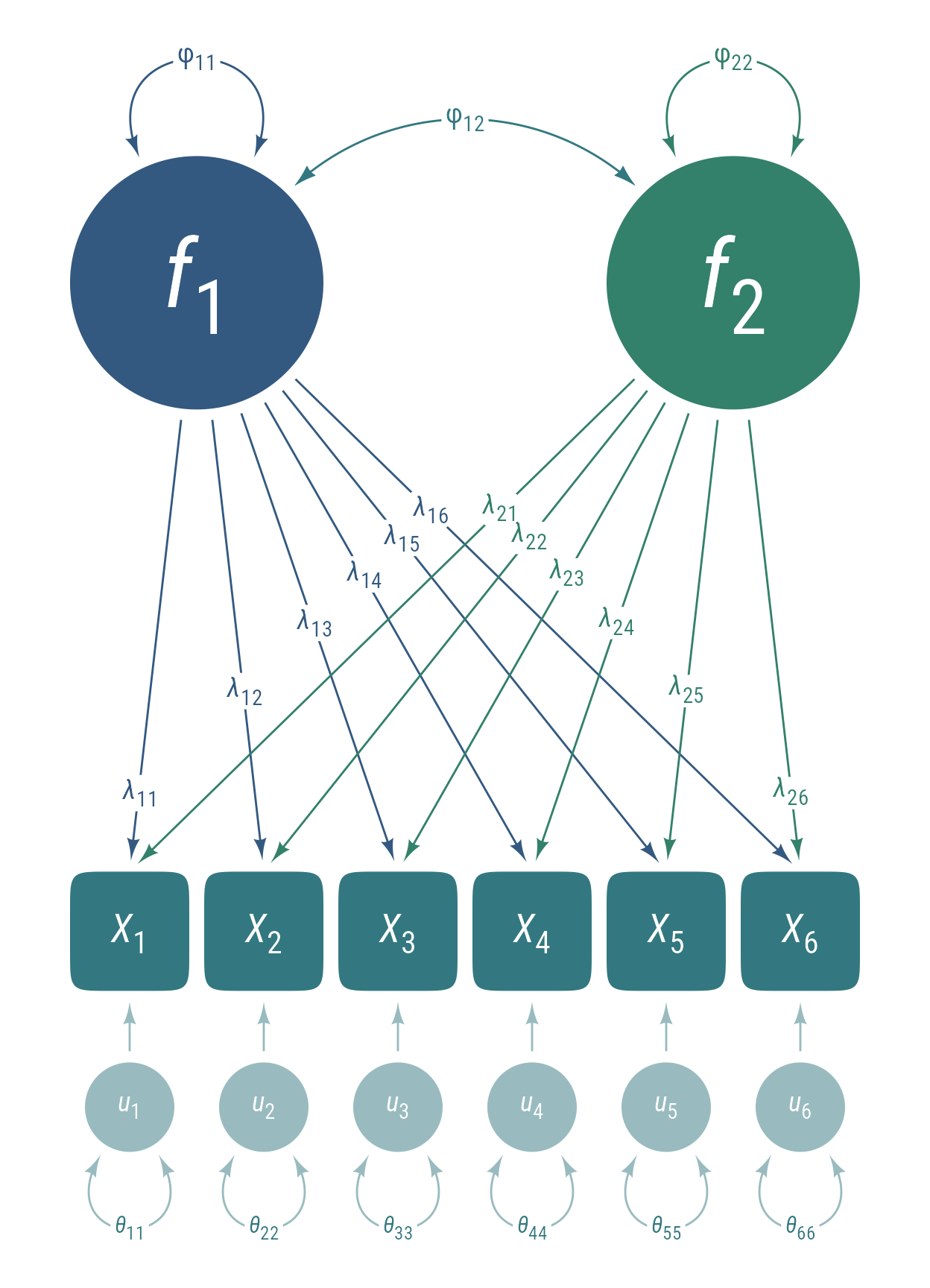
Exploratory factor analysis (EFA) assumes that observed variables intercorrelate because there is a smaller number of latent variables influence multiple observed variables. In Figure 6, there are 6 observed variables x that intercorrelate because 2 latent factors f act as common causes.
EFA will find the loadings from latent to observed variables that best account for the observed correlations among variables. Some portion of the observed variables is independent of the latent factors. These independent influences can be thought of as uniquenesses u. Thus, the structural model is:
where x is the vector observed variables, f is the vector of latent factors, u is the vector of latent uniquenesses, and Λ is the matrix of loadings that quantify the strength of the effects of f on x.
The observed variables x, latent factors f, and uniquenesses u each have their own covariance matrices:
The model-implied covariance matrix for the observed variables is a function of the loading matrix Λ and the covariance matrices Φ and Θ:
Code
my_fills <- viridis::viridis(n = 3, begin = .3, end = .6) |>
class_color() |>
set_props(saturation = .6, brightness = .5) |>
c()
ggdiagram(font_family = my_font, font_size = 16) +
{x <- ob_array(ob_ellipse(m1 = 8,
color = NA,
fill = my_fills[2]),
k = 6,
sep = .25)} +
ob_label(label = paste0("*X*~",1:6, "~"),
center = x@center,
size = 20,
fill = NA,
nudge_y = -.1,
color = "white") +
{f1 <- ob_circle(radius = x[1:2]@bounding_box@width / 2,
fill = my_fills[1],
color = NA,
label = ob_label(
"*f*~1~",
size = 48,
nudge_y = -.2,
fill = NA,
color = "white")) |>
place(from = midpoint(x[1], x[2]),
where = "above",
sep = x[1:4]@bounding_box@width)} +
{f2 <- ob_circle(radius = x[5:6]@bounding_box@width / 2,
fill = my_fills[3],
color = NA,
label = ob_label(
"*f*~2~",
size = 48,
nudge_y = -.2,
fill = NA,
color = "white")) |>
place(midpoint(x[5], x[6]),
where = "above",
sep = x[1:4]@bounding_box@width)} +
{f1x <- connect(f1,
x@north,
resect = 2,
color = my_fills[1])} +
{f2x <- connect(f2,
x@north,
resect = 2,
color = my_fills[3])} +
{a <- intersection(f1@tangent_at(45), f2@tangent_at(135))
ob_arc(center = a,
radius = distance(a, f1@point_at(45)),
start = (f1@point_at(45) - a)@theta,
end = (f2@point_at(135) - a)@theta,
color = my_fills[2],
resect = 2,
linewidth = .5,
arrowhead_length = 7,
arrow_head = arrowhead(),
arrow_fins = arrowhead(),
label = ob_label("φ~12~",
color = my_fills[2],
vjust = .5,
size = 14))} +
{ob_label(paste0("*λ*~2", 1:6, "~"),
intersection(f1x[6] + ob_point(1.2,0), f2x),
size = 14,
label.padding = margin(),
color = my_fills[3])} +
{ob_label(paste0("*λ*~1", 1:6, "~"),
intersection(f2x[1] + ob_point(-1.2,0), f1x),
size = 14,
label.padding = margin(t = 2, l = 2),
color = my_fills[1])} +
ob_variance(
x = f1,
color = my_fills[1],
label = ob_label("φ~11~", color = my_fills[1], size = 14)
) +
ob_variance(
x = f2,
color = my_fills[3],
label = ob_label("φ~22~", color = my_fills[3], size = 14)
) +
{u <- ob_circle(
radius = .75,
color = NA,
fill = my_fills[2],
alpha = .5,
label = ob_label(
paste0("*u*~", 1:6, "~"),
fill = NA,
color = "white",
size = 14
)
)@place(x, "below", sep = 1.2)} +
connect(u, x, color = my_fills[2], resect = 2) +
ob_variance(
u,
where = "south",
color = my_fills[2],
theta = 65,
looseness = 2.3,
label = ob_label(
paste0("*θ*~", 1:6 * 11, "~"),
color = my_fills[2],
label.margin = margin(),
size = 12
)
)
Path Diagrams for Principal Components Analysis
Principal components analysis (PCA) is similar to exploratory factor analysis (EFA) in that it finds latent factors from covariances among observed variables. The underlying model of PCA differs from EFA in that the indicators are formative rather than reflective. Because the principal components are fully determined by the observed variables, they have no error term. That is, they act as weighted summaries of the observed variables. In general, PCA creates latent variables that better summarize the observed data, and EFA creates latent variables that better approximate the underlying structure of the data.
Code
ggdiagram(font_family = my_font) +
  # observed variables
  {o <- ob_ellipse(m1 = 10, a = .6, color = NA) |>
      ob_array(5, sep = .2, fill = class_color(my_fills[2])@lighten(seq(.6, .9, length.out = 5)))} +
  # principal components
  {pc <- ob_circle(fill = my_fills[c(1,3)], color = NA) |>
    place(o[c(2, 4)], "above", 2)} +
  # direct effects from o to pc
  map(
    unbind(pc), \(pci) {
      connect(from = o@north,
              to = pci,
              color = pci@fill,
              resect = 2)@geom()
    }
  ) +
  # covariances among observed variables
  map(1:4, \(i) {
    offset <- c(-1.5, -.5, .5, 1.5) * .11
    ob_covariance(
      x = o[seq(i + 1, 5)]@south +
        ob_point(offset[seq(1, 5 - i)], 0),
      y = o[i]@south +
        ob_point(-offset[seq(1, 5 - i)], 0),
      bend = 45,
      looseness = 1.4,
      linewidth = .5,
      arrowhead_length = 6,
      color = my_fills[2]
    )@geom()
  }) +
  # Labels
  ob_label("Formative<br>Indicators", size = 16, fill = NA) |>
    place(o@bounding_box@east, sep = .8) +
  ob_label("Principal<br>Components", size = 24, fill = NA) |>
    place(pc@bounding_box@east, sep = 1.3) +
  # Invisible point to prevent label from clipping
  ob_point(o@bounding_box@east@x + 1.2, 1, color = "white")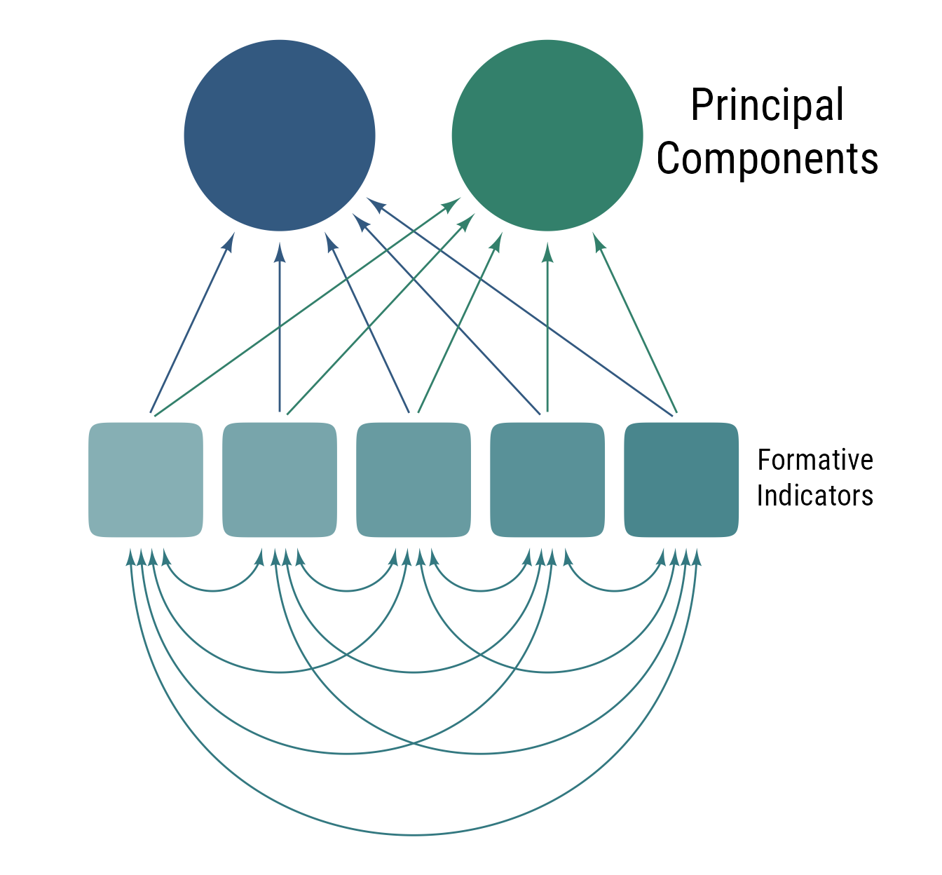
Path Diagrams for Confirmatory Factor Analysis
Figure 8 shows the primary ingredients of a latent variable model. Latent variables are not observed directly but are inferred from the correlations among observed variables. Latent variables are displayed as circles or ellipses. Their variances are depicted as curved double-headed arrows that circle back to the same latent variable. The observed variables from which latent variables are inferred are called indicator variables. The direct effects from a latent variable to its indicators are called loadings. The variability in indicator variables that is not explained by latent variables are explained by latent residuals (AKA errors). Each residual has its own variance. In some path diagrams, residual variances are affixed directly to observed variables, and the residual variables are omitted.
Code
ggdiagram(font_family = my_font, font_size = 16) +
  # Place a latent variable at the top
  {l1 <- ob_circle(radius = 2)} +
  # Place an array of observed variables below the circle
  {o3 <- ob_ellipse(m1 = 9) |>
    place(from = l1,
          where = "below",
          sep = 2) |>
    ob_array(
      k = 3,
      where = 0,
      sep = .4)} +
  # Connect the latent to the observed variables at the north anchor point
  {l1_o3 <- connect(l1,
                    o3@north,
                    resect = 2)} +
  # Place error terms below each observed variable
  {e3 <- ob_circle(radius = .75) |>
    place(o3,
          where = "below",
          sep = .85)} +
  # Connect the error terms to the observed variables
  {e3_o3 <- connect(e3, o3, resect = 2)} +
  # latent variance1
  {v_l1 <- ob_variance(l1, where = "north")} +
  # label(1, v_l1@midpoint()) +
  {v_e3 <- ob_variance(
    e3,
    where = "south",
    looseness = 1.4,
    resect = unit(3, "pt"),
    arrowhead_length = unit(7, "pt"),
    arrow_head = arrowhead(),
    arrow_fins = arrowhead())} +
  {lb_indicator <- ob_label("Indicator<br>Variables",
                            color = "black") |>
    place(o3[1]@west, "west", sep = 1.2)} +
  ob_point(-5, 0, color = "white") +
  ob_label("Loadings",
           lb_indicator@center %|-% midpoint(l1, o3@bounding_box)) +
  ob_label("Residuals",
           lb_indicator@center %|-% e3@bounding_box@center) +
  ob_label("Latent<br>Variable", lb_indicator@center %|-% l1) +
  ob_label("Latent<br>Variance",
           lb_indicator@center %|-% l1@normal_at(
             "north",
             distance = .5)) +
  ob_label("Residual<br>Variances",
           lb_indicator@center %|-% e3[1]@normal_at(
             "south",
             distance = .5))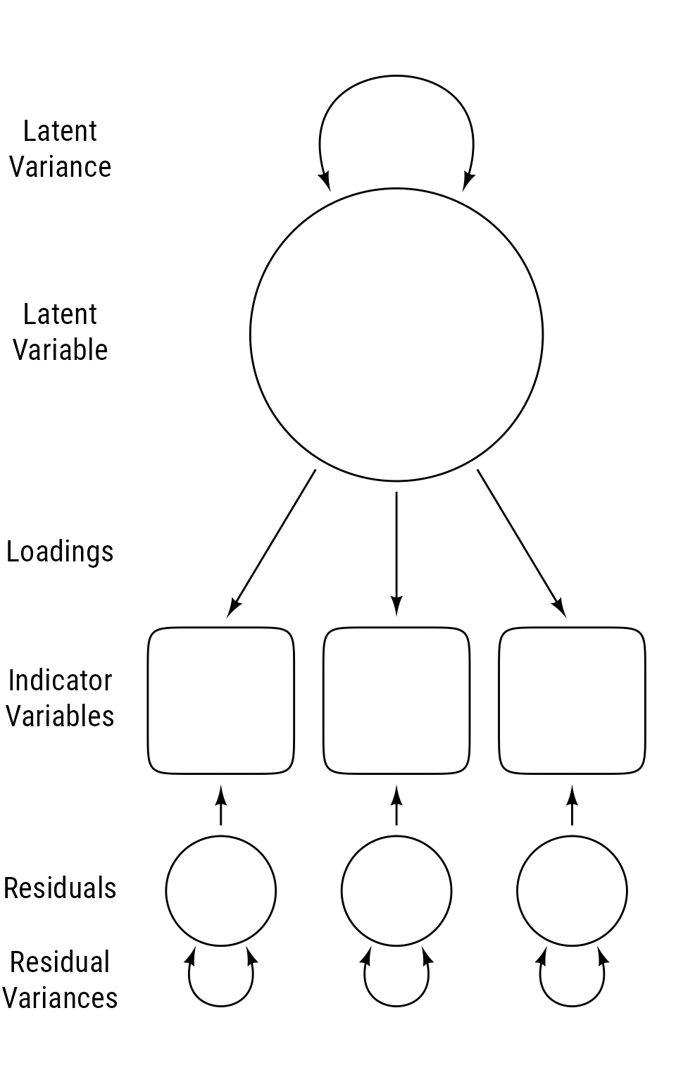
Code
my_fills <- viridis::viridis(n = 3, begin = .3, end = .6) |>
  class_color() |>
  set_props(saturation = .6, brightness = .5) |>
  c()

my_path_color <- "gray40"
my_resect <- 1
broad <- c("Gv", "Gf", "Gc")
g2broad <- c(Gv = .84, Gf = .95, Gc = .80)

broad2indicator <- list(Gv = c(.78, .84, .91),
                        Gf = c(.88, .81, .74),
                        Gc = c(.74, .91, .93))

broad_variance <- 1 - g2broad ^ 2

latent <- redefault(ob_circle,
                    color = NA)

lb_latent <- redefault(ob_label,
                            size = 30,
                            fill = NA,
                            color = "white")

observed <- redefault(ob_ellipse,
                           a = .5,
                           b = .5,
                           m1 = 10,
                           # fill = my_fill,
                           color = NA)

lb_observed <- redefault(
  ob_label,
  size = 15,
  fill = NA,
  color = "white",
  nudge_y = -.04)

direct <- redefault(
  connect,
  resect = my_resect,
  color = my_path_color,
  arrow_head = arrowhead(),
  linewidth = .5,
  length_head = 6
)

lb_direct <- redefault(
  ob_label,
  size = 16,
  color = lb_color,
  angle = 0,
  vjust = .5,
  position = .46,
  label.padding = margin(t = 3, r = 2, b = 0, l = 2, unit = "pt")
)

var_latent <- redefault(
  ob_variance,
  theta = 40,
  resect = my_resect,
  color = my_path_color,
  looseness = .9,
  linewidth = .5,
  arrow_head = arrowhead(),
  arrow_fins = arrowhead(),
  arrowhead_length = 6)

lb_variance <- redefault(
  lb_direct,
  position = .5,
  straight = TRUE
)

ggdiagram(font_family = my_font, font_size = 16) +
  {g <- latent(label = lb_latent("*g*"), fill = "gray15")} +
  var_latent(g, label = lb_variance(1)) +
  {Gx <- place(g, g,where = "below", sep = 1.6) |>
    ob_array(k = 3,
                sep = 2,
                label = lb_latent(broad,
                                  vjust = .6),
                fill = my_fills)} +
  var_latent(Gx,
             where = "left",
             color = Gx@fill,
             label = lb_variance(
               round_probability(broad_variance,
                                 phantom_text = "."),
               color = Gx@fill)) +
  {pGx <- direct(g, Gx, color = Gx@fill)} +
  {lb_direct(
    label = round_probability(g2broad,
                              phantom_text = "."),
    center = pGx@line@point_at_y(pGx[2]@midpoint(
      position = .47)@y),
    color = Gx@fill)} +
  # list----
  {vv <- map_ob(Gx, \(b) {
    o1 <- place(observed(fill = b@fill),
                from = b,
                where = "south",
                sep = 1.6)

    o <- ob_array(
      o1,
      k = 3,
      sep = .2,
      fill = purrr::map_chr(c(.6, .75, .9), tinter::lighten, x = o1@fill),
      label = lb_observed(
        paste0(
          b@label@label,
          "~",
          1:3,
          "~")))
    p <- direct(b, o@north, color = b@fill)

    l <- lb_direct(
      round_probability(
        broad2indicator[[b@label@label]],
        phantom_text = "."),
      center = p@line@point_at_y(p[2]@midpoint(position = .47)@y),
      color = b@fill)

    v <- ob_variance(
      o,
      where = "south",
      bend = -15,
      looseness = 1.7,
      resect = my_resect,
      color = b@fill,
      theta = 70,
      linewidth = .5,
      label = lb_variance(
        round_probability(sqrt(1 - broad2indicator[[b@label@label]] ^ 2)),
        color = b@fill),
      arrow_head = arrowhead(),
      arrow_fins = arrowhead(),
      arrowhead_length = 6
    )
    c(o, p, v, l)
  }) }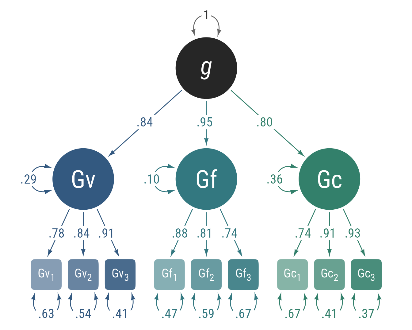
In Figure 10, the same model from Figure 9 is displayed showing variance proportions. The observed and latent variables all have an area of 1. The residual effects have areas proportional to their variances. The pie wedges in the endogenous latent variables and stacked bars in the observed variables have areas equal to the variance portions of their source variables.
Code
ggdiagram(font_family = my_font, font_size = 13) +
  {g <- latent(label = lb_latent("*g*"),
               fill = "gray15",
               radius = sqrt(1 / pi))} +
  {Gx <- place(g, g,where = "below", sep = 1.2) |>
    ob_array(k = 3,
                sep = 2.4,
                label = lb_latent(broad,
                                  vjust = .6,
                                  color = "gray15",
                                  size = 28),
                fill = "gray15")} +
  {d_Gx <- ob_circle(
    color = NA,
    fill = my_fills,
    radius = sqrt(broad_variance / pi)) |>
    place(Gx, where = "left", sep = .45)} +
  direct(d_Gx,
          Gx,
          color = my_fills,
          resect = 1) +
  {pGx <- direct(g, Gx, color = Gx@fill, resect = 1)} +
  {lb_direct(
    label = round_probability(g2broad,
                              phantom_text = "."),
    center = pGx@line@point_at_y(pGx[2]@midpoint(
      position = .46)@y),
    color = Gx@fill)} +
  ob_wedge(center = Gx@center,
           radius = sqrt(1 / pi),
           start = turn(.5) + turn(broad_variance) / 2,
           end = turn(.5) - turn(broad_variance) / 2,
           fill = my_fills) +
  lb_latent(broad, center = Gx@center, vjust = .6) +
  {map(1:3, \(i) {
    b <- Gx[i]
    p2 <- place(ob_point(), from = b, where = "south", sep = 1.2)
    p1 <- place(ob_point(), from = p2, where = "left", sep = 1.1)
    p3 <- place(ob_point(), from = p2, where = "right", sep = 1.1)

    p <- bind(c(p1,p2,p3))

    b_text <- b@label@label

    lb_o <- ob_label(paste0(b_text, "~", 1:3, "~"),
                     center = p - ob_point(0,.55),
                     color = "white",
                     size = 20,
                     fill = NA)


    b_p <- direct(b, p, color = my_fills[i], resect = 1)

    l_b_p <- lb_direct(
      round_probability(broad2indicator[[b_text]],
                        phantom_text = "."),
      center = b_p@line@point_at_y(b_p[2]@midpoint(.46)@y),
      color = my_fills[i])

    r_g <- ob_rectangle(
      north = p,
      fill = g@fill,
      color = NA,
      width = 1,
      height = (g2broad[b_text] * broad2indicator[[b_text]]) ^ 2)

    r_broad <- ob_rectangle(
      north = r_g@south,
      fill = my_fills[i],
      width = 1,
      color = NA,
      height = (sqrt(broad_variance[b_text]) * broad2indicator[[b_text]]) ^ 2)

    error_variance <- 1 - broad2indicator[[b_text]] ^ 2

    error_color <- class_color(my_fills[i])@lighten(.5)@color

    r_unique <- ob_rectangle(
      north = r_broad@south,
      fill = error_color,
      width = 1,
      color = NA,
      height = error_variance)

    r <- sqrt(error_variance / pi)

    error <- ob_circle(r_unique@south - ob_point(0, r + .45), radius = r, color = NA, fill = error_color)

    error2observed <- direct(error, r_unique, resect = 1, color = error_color)

    list(r_g,
         r_broad,
         r_unique,
         b_p,
         l_b_p,
         error,
         error2observed,
         lb_o) |>
      lapply(as.geom)
  })}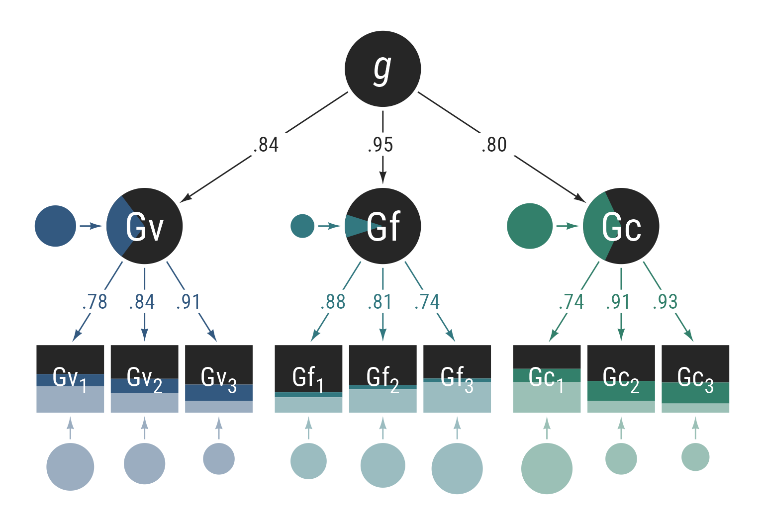
Figure 11 is a demonstration of how ggdiagram can be used to creating complex models with an eye to aesthetics.
Code
my_serif_font <- "Equity Text A"
str_narrow <- "Narrow Abilities"
str_tests <- "Tests"
str_specifics <- "Specifics"

# gradient fills
black_gradient <- grid::radialGradient(
  colours = rev(c("gray50", "gray2", "gray2")),
  stops = c(0, .35, 1), group = FALSE)
black_gradient_rev <- grid::radialGradient(
  colours = c("gray50", "black"), group = FALSE)

ggdiagram(font_family = my_serif_font, font_size = 16) +
  {g <- ob_circle(
      radius = 1.33,
      fill = NA,
      color = NA
    )} +
  geom_polygon(
    aes(x = x, y = y),
    data = ob_circle(radius = 9)@polygon,
    color = NA,
    fill = black_gradient) +
  geom_polygon(
    aes(x = x, y = y),
    data = g@polygon,
    color = NA,
    fill = black_gradient_rev) +
  {broad_angle <- turn(seq(0, 1, length.out = 9)[-9] + 1 / 16)
   broad_color <- hcl(
     h = seq(0, 360 - 360 / 8, 360 / 8) + 20,
     c = 55,
     l = 60)
    broad <- ob_circle(
      color = NA,
      fill = broad_color) |>
      place(
        from = g,
        where = broad_angle,
        sep = 1.15)} +
  ob_label(
        "*g*",
        color = "gray90",
        fill = NA,
        size = 60,
        vjust = .4,
        family = my_serif_font
      ) +
  connect(g, broad,
          color = broad_color,
          resect = 1,
          linewidth = .75,
          length_head = 5) +
  purrr::map(unbind(broad), \(b) {
    geom_polygon(
      data = b@polygon,
      aes(x = x, y = y),
      fill = grid::radialGradient(
        colours = c(tinter::lighten(b@fill, .4),
                    tinter::lighten(b@fill, .8)),
        stops = c(0,1),
        group = FALSE))}) +
  ob_label(
    c("Ga", "Gc", "Gf", "Gv", "Gs", "Gr", "Gl", "Gwm"),
    broad@center + ob_point(0, -.05),
    fill = NA,
    family = my_serif_font,
    size = 20,
    vjust = .55,
    angle = broad@center@theta + degree(-90 * sign(broad@center@theta@turn)),
    color = "gray20"
  ) +
  ob_path(
    broad |>
      set_props(radius = c(rep(.66, 4), rep(.59, 4))) |>
      unbind() |>
      purrr::map(\(x) {
        x@point_at(x@center@theta + degree(seq(-90, 90, 10)))
        }),
    color = "gray20",
    alpha = 0,
    label = ob_label(
      c("Auditory",
        "Knowledge",
        "Fluid",
        "Visual-Spatial",
        "Speed",
        "Fluency",
        "Efficiency",
        "Memory"),
      fill = NA,
      family = my_serif_font,
      vjust = 1,
      size = 9.5,
      spacing = 100)) +
  ob_path(
    broad |>
      set_props(radius = c(rep(.59, 4), rep(.66, 4))) |>
      unbind() |>
      purrr::map(\(x) {
        x@point_at(
          x@center@theta + degree(-180) + degree(seq(-90, 90, 10)))}),
    label = ob_label(
      c("Processing",
        "Comprehension",
        "Reasoning",
        "Processing",
        "Processing",
        "Retrieval",
        "Learning",
        "Working"),
            fill = NA,
            family = my_serif_font,
            vjust = 1,
      size = 9.5,
            spacing = 100
          ),
          color = "gray20",
          alpha = 0
  ) +
  {narrow <- ob_circle(
    radius = .45,
    fill = rep(broad@fill, each = 5)
    ) |>
    place(from = g,
          where = degree(seq(0, 360 - 360/40, 360/40) + 360/80),
          sep = 4.3)

    geom_polygon(
      aes(x = x,
          y = y,
          group = group,
          fill = fill),
      data = narrow@polygon,
      color = NA)} +
  {purrr::imap(unbind(broad), \(x, idx) {
    connect(x, narrow[(idx - 1) * 5 + 1:5],
            color = tinter::lighten(x@fill, .5),
            linewidth = .5,
            length_head = 6,
            resect = 1) |>
      as.geom()
  })} +
  {test_theta <- degree(seq(0, 360 - 360/120, 360/120) + 360/240)
    tests <- ob_ellipse(
      a = .18,
      m1 = 8,
      angle = test_theta,
      color = NA,
      fill = rep(tinter::lighten(broad@fill, .2), each = 15)) |>
      place(from = g, where = test_theta, sep = 6.2)} +
  {specifics <- ob_circle(
    radius = .2,
    angle = test_theta,
    color = NA,
    fill = rep(tinter::lighten(broad@fill, .15), each = 15)) |>
    place(from = g, where = test_theta, sep = 7.0)} +
  connect(specifics, tests,
          color = specifics@fill,
          linewidth = .3,
          length_head = 6,
          resect = .5) +
  {purrr::imap(unbind(narrow), \(x, idx) {
    connect(x, tests[(idx - 1) * 3 + 1:3],
            color = tinter::lighten(x@fill, .5),
            resect = 1,
            linewidth = .3,
            length_head = 6) |>
      as.geom()
  })} +
  scale_fill_manual(
    values = map(broad@fill,
                 \(fill) {
                   grid::radialGradient(c(tinter::lighten(fill, .15),
                                          tinter::lighten(fill, .4)),
                                        stops = c(0.2, 1),
                                        group = FALSE)}) |>
      `names<-`(broad@fill)) +
  theme(legend.position = "none") +
  ob_label(
    label = rev(strsplit(str_narrow, split = character(0))[[1]]),
    center = narrow[seq(nchar(str_narrow)) + 2]@center,
    angle = narrow[seq(nchar(str_narrow)) + 2]@center@theta - degree(90),
    fill = NA,
    family = my_serif_font,
    size = 16,
    color = "gray30",
    vjust = .55
  ) +
  ob_label(
    label = strsplit(str_narrow, split = character(0))[[1]],
    center = narrow[seq(nchar(str_narrow)) + 22]@center,
    angle = narrow[seq(nchar(str_narrow)) + 22]@center@theta + degree(90),
    fill = NA,
    family = my_serif_font,
    size = 16,
    color = "gray30",
    vjust = .55
  ) +
  {purrr::map(65 + c(0,15, 30, 45), \(x) {
    ob_label(
      label = strsplit(str_tests, split = character(0))[[1]],
      center = tests[seq(nchar(str_tests)) + x]@center,
      angle = tests[seq(nchar(str_tests)) + x]@center@theta + degree(90),
      fill = NA,
      family = my_serif_font,
      size = 10,
      color = "gray30",
      vjust = .57
    )@geom()
  })} +
  {purrr::map(5 + c(0,15, 30, 45), \(x) {
    ob_label(
      label = rev(strsplit(str_tests, split = character(0))[[1]]),
      center = tests[seq(nchar(str_tests)) + x]@center,
      angle = tests[seq(nchar(str_tests)) + x]@center@theta - degree(90),
      fill = NA,
      family = my_serif_font,
      size = 10,
      color = "gray30",
      vjust = .57
    )@geom()})} +
  {purrr::map(63 + c(0,15, 30, 45), \(x) {
    ob_label(
      label = strsplit(str_specifics, split = character(0))[[1]],
      center = specifics[seq(nchar(str_specifics)) + x]@center,
      angle = specifics[seq(nchar(str_specifics)) + x]@center@theta + degree(90),
      fill = NA,
      family = my_serif_font,
      size = 9,
      color = "gray30",
      vjust = .53
    )@geom()})} +
  {purrr::map(3 + c(0,15, 30, 45), \(x) {
    ob_label(
      label = rev(strsplit(str_specifics, split = character(0))[[1]]),
      center = specifics[seq(nchar(str_specifics)) + x]@center,
      angle = specifics[seq(nchar(str_specifics)) + x]@center@theta - degree(90),
      fill = NA,
      family = my_serif_font,
      size = 9,
      color = "gray30",
      vjust = .53
    )@geom()})}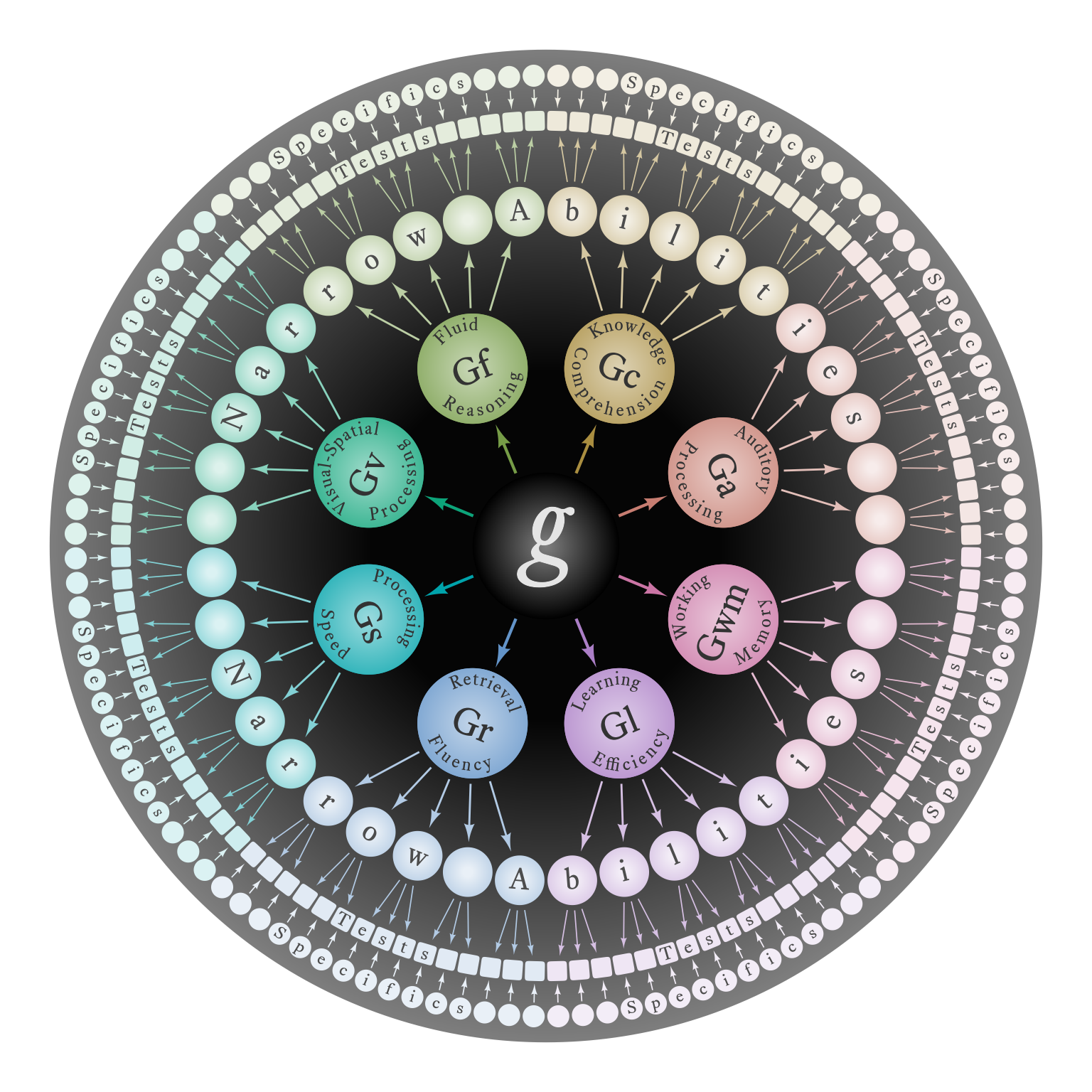
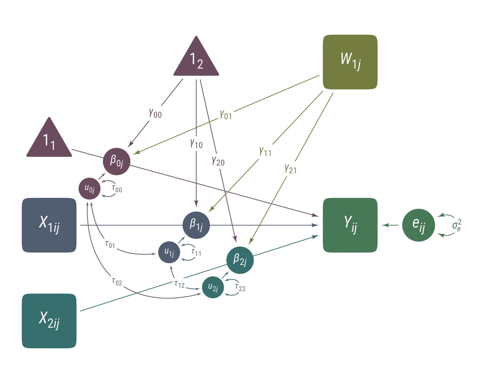
Path Diagrams for Multilevel Models
The independence assumption of multiple regression requires that the regression errors are independent of each other. When data are clustered in some way that violates this assumption, a multilevel model can account for the within-cluster similarity of data (i.e., the intraclass correlation). Most multilevel models are displayed with equations like these:
Here we have an outcome (Y), 2 level-1 predictors (X1 and X2), and 1 level-2 predictor (W1). The random intercept (β0j) has as fixed component (γ00 + γ01W1j) and a random component (u0j). The random intercept is partly predicted by the level-2 variable, W1j. The random slopes also have fixed and random components, as well as being predicted by the level-2 variable. The τ matrix is variance-covariance matrix of the level-2 random variables u (i.e., u0j, u1j, and u1j).
These equations specify the model unambiguously, but it is easy to lose one’s way in them. It can facilitate interpretation if the equations are presented in a visual mode.
Curran & Bauer (2007) developed a set of extensions to path diagrams to incorporate random slopes and intercepts from multilevel models. Their core innovation is to treat random slopes and intercepts as latent variables that sit atop direct paths. An example of this approach is in Figure 12. It displays the same information as the equations listed previously, but in terms that are easier to understand and use.
Code
clr <- class_color(
c("#976A85",
"#7385A1",
"#4E9C9B",
"#66AB7A",
"#A4AF5A"))@darken(.3)@color
clr <- c("#6B4B5E", "#515E72", "#376E6E", "#487956", "#747C3F")
observed <- redefault(ob_ellipse, m1 = 10, color = NA)
lb_observed <- redefault(ob_label, fill = NA, color = "white", size = 24)
lb_slope <- redefault(ob_label, fill = NA, color = "white", size = 18)
random_slope <- redefault(ob_circle, color = NA, radius = .5)
tau_covariance <- redefault(ob_covariance,
linewidth = .5,
head_length = 4,
resect = 1)
latent_slope_line <- ob_line(slope = -.8, intercept = 1.3)
ggdiagram(font_family = my_font, font_size = 13) +
{i1 <- ob_intercept(
width = 2,
label = ob_label(
label = "1~1~",
color = "white",
fill = NA,
size = 24),
vertex_radius = unit(.6, "mm"),
fill = clr[1])} +
{x1 <- observed(label = lb_observed("*X*~1*ij*~"),
fill = clr[2]) |>
place(from = bind(i1@segment)@midpoint()[2],
where = "below",
sep = 1.5)} +
{x2 <- observed(label = lb_observed("*X*~2*ij*~"),
fill = clr[3]) |>
place(from = x1,
where = "below",
sep = 1.5)} +
{y <- observed(label = lb_observed("*Y*~*ij*~"),
fill = clr[4]) |>
place(from = x1,
where = "right",
sep = 9)} +
{i1_y <- connect(i1, y, resect = 2, color = clr[1])} +
{x1_y <- connect(x1, y, resect = 2, color = clr[2])} +
{x2_y <- connect(x2, y, resect = 2, color = clr[3])} +
{latent_slope_line <- ob_line(slope = -.8, intercept = 1.3)
b0j <- random_slope(
intersection(latent_slope_line, i1_y@line),
fill = clr[1],
label = lb_slope("*β*~0*j*~")
)} +
{b1j <- random_slope(
intersection(latent_slope_line, x1_y@line),
fill = clr[2],
label = lb_slope("*β*~1*j*~"))} +
{b2j <- ob_circle(
intersection(latent_slope_line, x2_y@line),
radius = .5,
fill = clr[3],
color = NA,
label = lb_slope("*β*~2*j*~")
)} +
{i2 <- ob_intercept(width = 2,
rotate(latent_slope_line, degree(90), origin = b0j@center)@point_at_x(b1j@center@x),
label = lb_observed("1~2~"),
fill = clr[1],
vertex_radius = unit(.6, "mm")
)} +
{w1 <- observed(
center = i2@center %-|% y@center,
label = lb_observed("*W*~1*j*~"),
fill = clr[5]
)} +
{b <- bind(c(b0j, b1j, b2j))
i2b <- connect(
i2,
b,
color = i2@fill,
resect = 2,
label = ob_label(
paste0("*γ*~", 0:2, "0~"),
angle = 0,
size = 16
)
)} +
{w1b <- connect(
w1,
b,
color = w1@fill,
resect = 2,
label = ob_label(
paste0("*γ*~", 0:2, "1~"),
angle = 0,
size = 16
)
)} +
{u <- ob_circle(
radius = .4,
color = NA,
fill = b@fill,
label = ob_label(
paste0("*u*~", 0:2, "*j*~"),
color = "white",
fill = NA,
size = 14
)
) |> place(b, "southwest", .5)} +
connect(
u,
b,
color = b@fill,
resect = 1,
length_head = 4,
linewidth = .5
) +
tau_covariance(
u[2],
u[1],
color = mean_color(clr[c(1, 2)]),
label = ob_label("*τ*~01~",
color = mean_color(clr[c(1, 2)]))
) +
tau_covariance(
u[3],
u[2],
color = mean_color(clr[c(2, 3)]),
label = ob_label("*τ*~12~", color = mean_color(clr[c(2, 3)]))
) +
tau_covariance(
u[3]@point_at(210),
u[1]@point_at(260),
color = mean_color(clr[c(1, 3)]),
label = ob_label("*τ*~02~", color = mean_color(clr[c(1, 3)])),
bend = 10
) +
ob_variance(
u,
color = u@fill,
"east",
linewidth = .5,
looseness = 1.9,
bend = 5,
arrowhead_length = 4,
resect = 1,
label = ob_label(
paste0("*τ*~", 0:2, 0:2, "~"),
label.margin = margin(),
label.padding = margin(),
color = b@fill
),
theta = 60
) +
{e <- ob_circle(radius = .6, fill = y@fill, color = NA, label = lb_observed("*e~ij~*")) |> place(y, "right", .9)} +
connect(e, y, color = y@fill, resect = 2) +
{e_var <- ob_variance(e, "east", color = e@fill, looseness = 1.7)} +
ob_latex(r"(\text{\emph{σ}}^{\text{2}}_{\mkern-1.5mu\text{\emph{e}}})", e_var@midpoint(), width = .45, family = "Roboto Condensed", filename = "sigma_e_2", color = e@fill)
Path Models for Bivariate Latent Growth Models
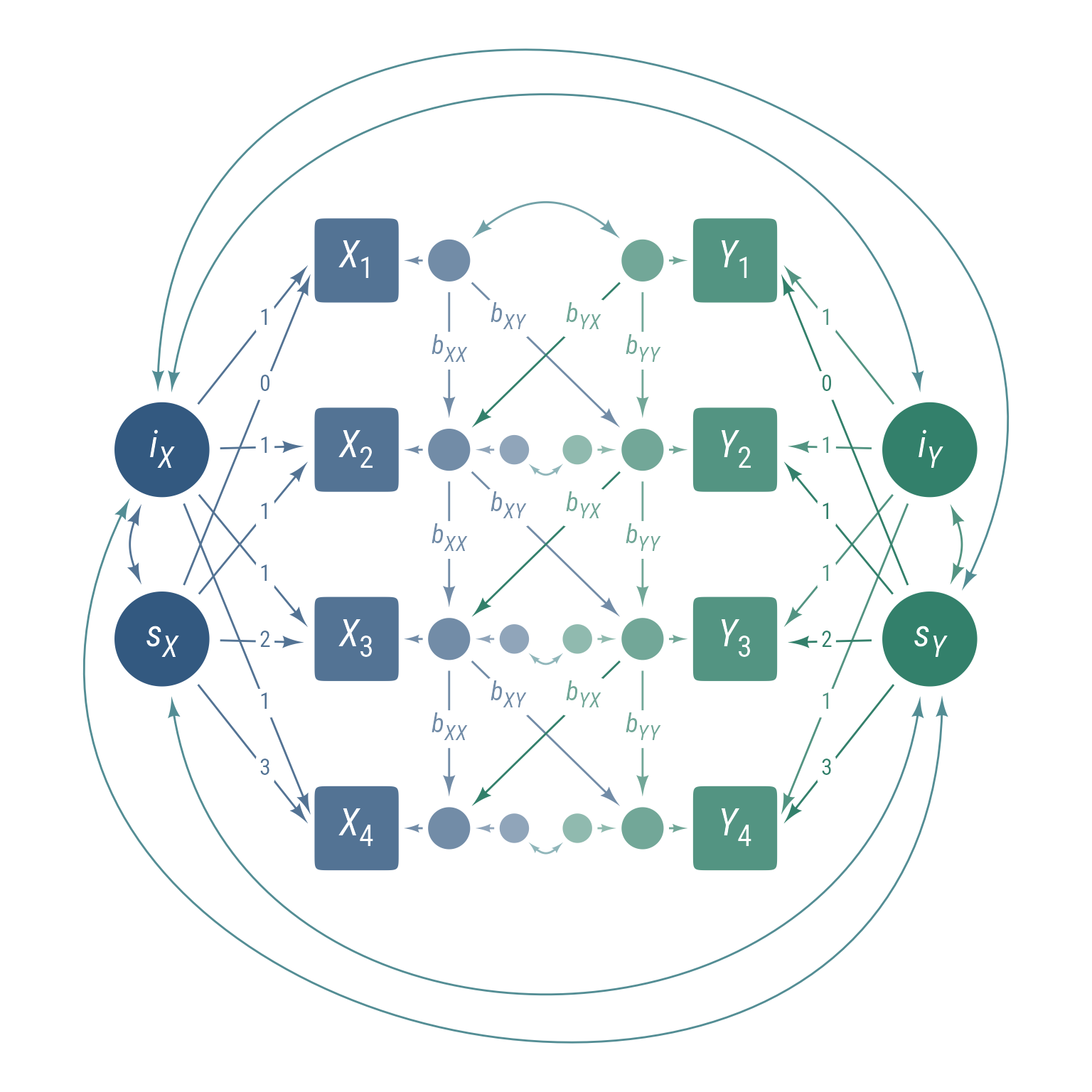
Bivariate latent growth models are used to model the change in two variables over time. The latent intercepts iX and iY represent the initial status of the two variables, while the latent slopes sX and sY represent the linear growth rate. The model also includes structured residuals that allow for the separation of between-person change and within-person change Curran et al. (2014). The bXX and bYY autocorrelation parameters measures within-person stability, and the bXY and bYX cross-lag parameters measures within-person bidirectional influence.
Code
color_x <- class_color(my_fills[1])
color_y <- class_color(my_fills[3])
color_xy <- class_color(my_fills[2])
my_observed <- redefault(ob_ellipse,
                         m1 = 15,
                         fill = color_x@lighten(.85),
                         color = NA)

my_latent <- redefault(ob_circle,
                       radius = sqrt(4 / pi),
                         fill = color_x,
                         color = NA)

my_label <- redefault(
  ob_label,
  color = "white",
  fill = NA,
  size = 20,
  family = my_font,
  nudge_y = -.05
)
my_connect <- redefault(connect,
                        resect = 2,
                        color = color_x@lighten(.85))
my_connect2 <- redefault(connect,
                         length_head = 5,
                         resect = 1,
                         color = color_x@lighten(.70))
my_error <- redefault(ob_circle,
                      radius = .35,
                      fill = color_x@lighten(.7),
                      color = NA)
my_font <- "Roboto Condensed"
k <- 4
my_sep <- 2.5
e_sep <- .7
l_dist <- .53

ggdiagram(font_family = my_font, font_size = 24) +
  {x <- my_observed() |>
    ob_array(k,
             sep = 2.5,
             where = "south",
             label = my_label(paste0("*X*~" , 1:k, "~")))} +
  {y <- my_observed(label = my_label(paste0("*Y*~", 1:k, "~")),
                    fill = color_y@lighten(.85)) |>
    place(x, "right", sep = 7)} +
  {e_x <- my_error(radius = .5) |> place(x, "right", sep = e_sep)} +
  {e_y <- my_error(radius = .5,
                   fill = color_y@lighten(.70)) |>
    place(y, "left", sep = e_sep)} +
  {ee_x <- my_error(fill = color_x@lighten(.55)) |> place(e_x[-1], "right", sep = e_sep)} +
  {ee_y <- my_error(fill = color_y@lighten(.55)) |> place(e_y[-1], "left", sep = e_sep)} +
  {lxx <- my_connect(e_x[-k], e_x[-1], color = color_x@lighten(.70))} +
  ob_label("*b~XX~*", lxx@midpoint(.47), size = 14) +
  {lxy <- my_connect(e_x[-k], e_y[-1], color = color_x@lighten(.70))} +
  ob_label("*b~XY~*", lxy@midpoint(.27, color = color_x@lighten(.70)), size = 14) +
  {lyx <- my_connect(e_y[-k], e_x[-1], color = color_y)} +
  ob_label("*b~YX~*", lyx@midpoint(.27, color = color_y@lighten(.70)), size = 14) +
  {lyy <- my_connect(e_y[-k], e_y[-1], color = color_y@lighten(.70))} +
  ob_label("*b~YY~*", lyy@midpoint(.47), size = 14) +
  my_connect2(e_x, x, color = color_x@lighten(.70)) +
  my_connect2(e_y, y, color = color_y@lighten(.70)) +
  my_connect2(ee_x, e_x[-1], color = color_x@lighten(.55)) +
  my_connect2(ee_y, e_y[-1], color = color_y@lighten(.55)) +
  ob_covariance(e_x[1], e_y[1], color = color_xy@lighten(.70)) +
  ob_covariance(ee_y, ee_x,
                resect = 1,
                length_head = 4,
                length_fins = 4,
                looseness = 1.3,
                color = color_xy@lighten(.55)) +
  {ix <- my_latent(label = my_label("*i*~*X*~")) |>
    place(x[2]@point_at("left"), "left",
          sep = my_sep)} +
  {iy <- my_latent(label = my_label("*i*~*Y*~"),
                   fill = color_y) |>
    place(y[2]@point_at("right"),
          where = "right",
          sep = my_sep)} +
  {sx <- my_latent(label = my_label("*s*~*X*~")) |>
    place(x[3]@point_at("left"),
          where = "left",
          sep = my_sep)} +
  {sy <- my_latent(label = my_label("*s*~*Y*~"), fill = color_y) |>
    place(y[3]@point_at("right"), "right", sep = my_sep)} +
  {lx <- my_connect(ix, x@point_at(degree(175)))} +
  {ly <- my_connect(iy, y@point_at(degree(5)), color = color_y@lighten(.85))} +
  ob_label("1",
           center = lx@line@point_at_x(lx[2]@midpoint(l_dist)@x),
           size = 12) +
  ob_label("1",
           center = ly@line@point_at_x(ly[2]@midpoint(l_dist)@x),
           size = 12) +
  {lsx <- my_connect(sx, x@point_at(degree(185)))} +
  {lsy <- my_connect(sy, y@point_at(degree(-5)), color = color_y)} +
  ob_label(0:3,
           center = lsx@line@point_at_x(lsx[3]@midpoint(l_dist)@x),
           size = 12) +
  ob_label(0:3,
           center = lsy@line@point_at_x(lsy[3]@midpoint(l_dist)@x),
           size = 12) +
  ob_covariance(ix@point_at(degree(80)),
                iy@point_at(degree(100)),
                looseness = 1.1,
                bend = 40,
                color = color_xy@lighten(.85)) +
  ob_covariance(ix@point_at(degree(95)),
                sy@point_at(degree(55)),
                looseness = 1.5,
                bend = 60,
                color = color_xy@lighten(.85)) +
  ob_covariance(sy@point_at(degree(260)),
                sx@point_at(degree(280)),
                looseness = 1.1,
                bend = 40,
                color = color_xy@lighten(.85)) +
  ob_covariance(sy@point_at(degree(285)),
                ix@point_at(degree(235)),
                looseness = 1.5,
                bend = 60,
                color = color_xy@lighten(.85)) +
  ob_covariance(iy@point_at(degree(-70)),
                sy@point_at(degree(70)),
                bend = degree(-20),
                color = color_y@lighten(.85)) +
  ob_covariance(sx@point_at(degree(110)),
                ix@point_at(degree(-110)),
                bend = degree(-20),
                color = color_x@lighten(.85))