Setup
Base Plot
To avoid repetitive code, we set defaults and make a base plot:
my_font <- "Roboto Condensed"
my_font_size <- 20
my_point_size <- 2

# my_colors <- viridis::viridis(2, begin = .25, end = .5)
my_colors <- c("#3B528B", "#21908C")

theme_set(
  theme_minimal(
    base_size = my_font_size,
    base_family = my_font) +
    theme(axis.title.y = element_text(angle = 0, vjust = 0.5)))

bp <- ggdiagram(
  font_family = my_font,
  font_size = my_font_size,
  point_size = my_point_size,
  linewidth = .5,
  theme_function = theme_minimal,
  axis.title.x =  element_text(face = "italic"),
  axis.title.y = element_text(
    face = "italic",
    angle = 0,
    hjust = .5,
    vjust = .5)) +
  scale_x_continuous(labels = signs_centered,
                     limits = c(-4, 4)) +
  scale_y_continuous(labels = signs::signs,
                     limits = c(-4, 4))
Bézier curves
The ob_bezier function creates an object that specifies the control points for a bézier curve. A bézier curve is an extremely useful way of making elegantly curved lines between points.
bp +
  {control_points <- ob_point(
    x = c(-4,4,4),
    y = c(4,-4, 0))} +
  ob_path(control_points, linetype = "dashed", linewidth = .25) +
  ob_bezier(control_points)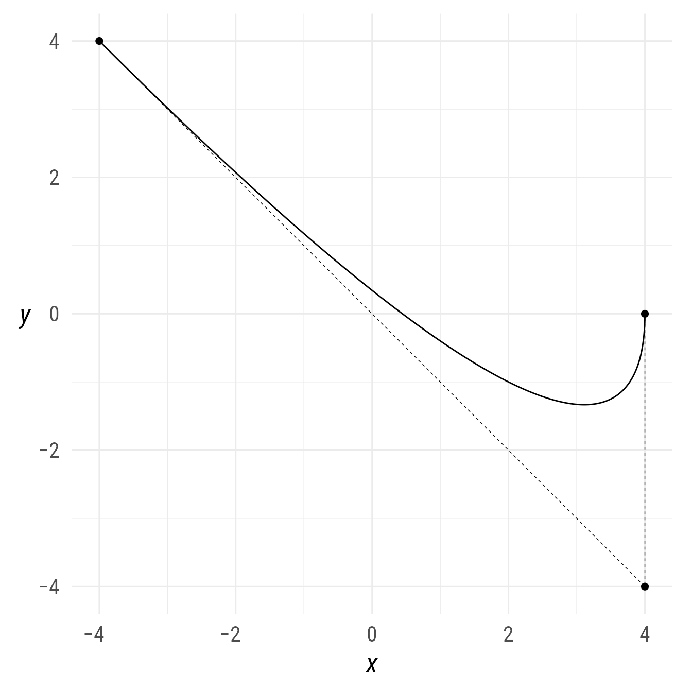
I like to make a list of control points setting the start and end points first. Then I find internal control points by offsetting from the end points—adding or subtracting a point at a specified x and y distance (or angle using the polar function).
The c function creates a list of all the points, and the bind function binds the list into a single point object containing all the points.
# start and end of control points
p_start <- ob_point(-4,-2)
p_end <- ob_point(4, 2)
# Offset ob_point from the endpoints
p_offset <- ob_point(5,6)

# Make list of points and bind them into a single ob_point
p <- c(p_start,
       p_start + p_offset,
       p_end - p_offset,
       p_end) |>
  bind()

bp +
  ob_path(p,
       linetype = "dashed",
       color = "gray",
       linewidth = .25) +
  p +
  ob_bezier(p,
label = ob_label("Labels can follow the path of the bézier curve.")) 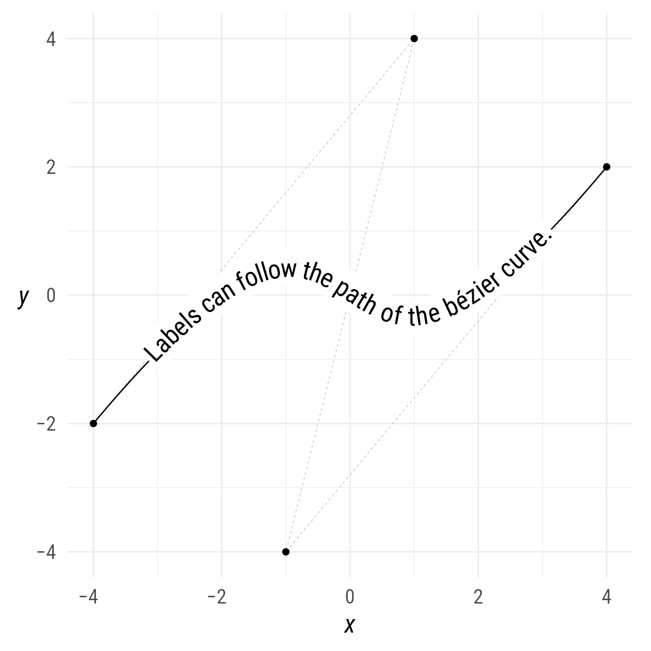
Multiple bézier paths
If multiple point objects are supplied as a list (or concatenated with the c function), a bézier curve will be created for each point object in the list.
control_point_list <- c(
      ob_point(
        x = c(-4, -3, 4),
        y = c(.1,  4, .1),
        color = my_colors[1]),
      ob_point(
        x = c(-4, 3, 4),
        y = c(-.1, -4, -.1),
        color = my_colors[2] )
      )
bp +
  ob_bezier(control_point_list) +
  ob_path(control_point_list, linetype = "dashed", linewidth = .25) +
  bind(control_point_list)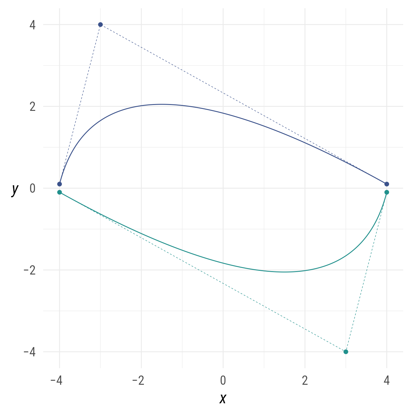
Curved Connectors
Drawing connectors between shapes is usually with straight line segments. However, a bezier curve with endpoints at the center of the objects can be drawn with a control point from the first object (from_offset) and/or a control point from second object (to_offset). These control points are relative to the endpoints, so from_offset = ob_point(1, 0) would be one unit to the right of the from endpoint, and to_offset = ob_polar("north", 1) would be one unit above the to endpoint.
ggdiagram(font_family = "Roboto Condensed",
          font_size = 18) +
  {A <- ob_rectangle(width = sqrt(pi),
                     height = sqrt(pi))} +
  {B <- ob_ngon(n = 8,
                color = "black",
                fill = NA,
                radius = 1.1) %>%
    place(A, "southeast")} +
  {C <- ob_circle() %>%
    place(B, "southeast")} +
  connect(A, B, resect = 2) +
  connect(B, C, resect = 2) +
  {AC <- connect(A,
                 C,
                 from_offset = ob_polar("south", 3),
                 to_offset = ob_polar("west", 3),
resect = 2)} 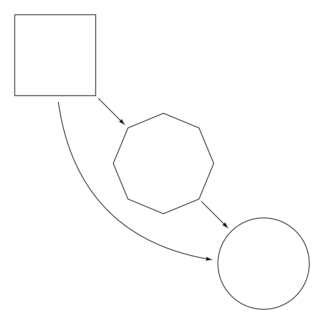
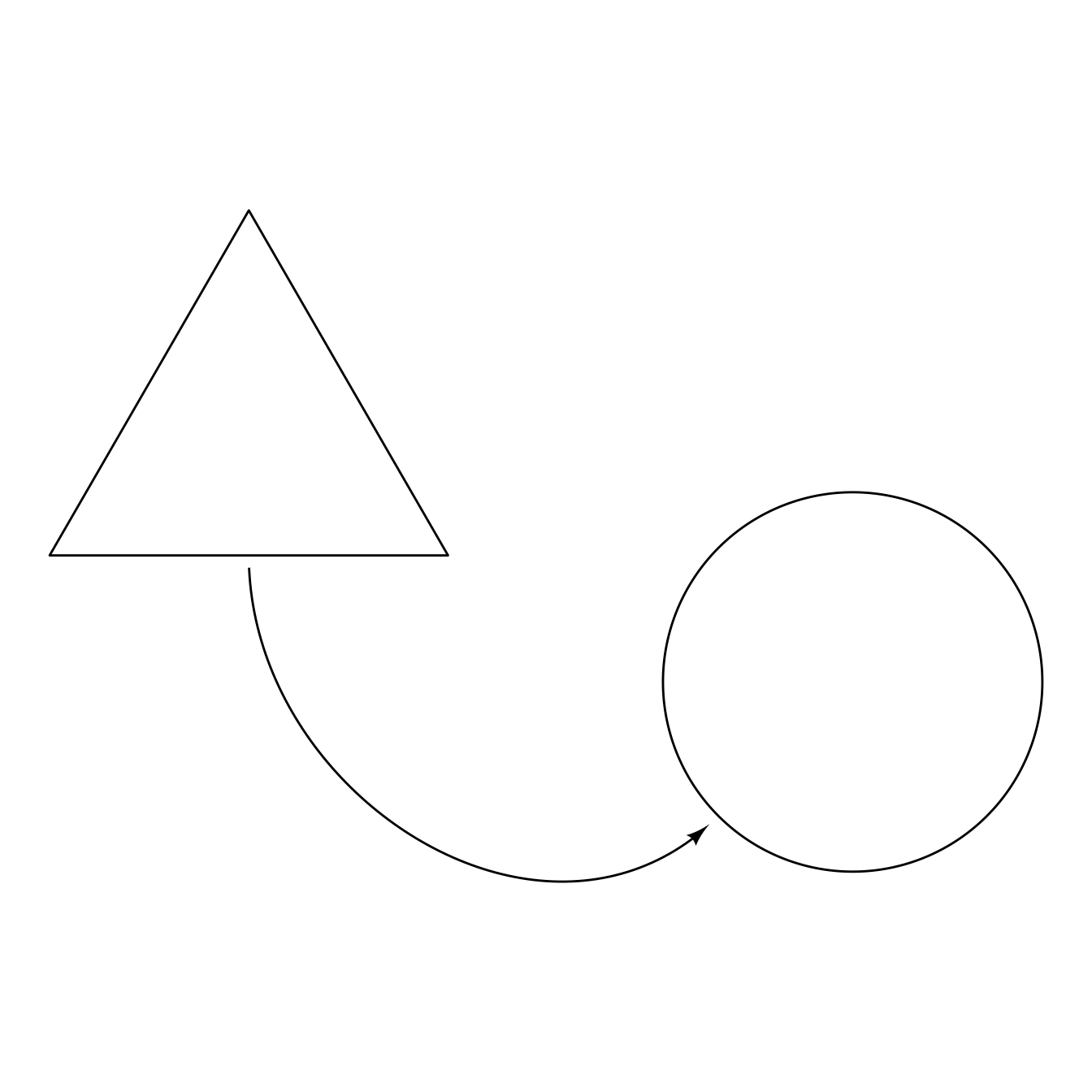
Of course, if you want the endpoints to be placed on some part of the shapes other than their centers, you can specify them directly. Here we specify that the curve start the south anchor point of a rectangle and end at the southwest point of a circle.
ggdiagram(font_family = "Roboto Condensed",
          font_size = 18) +
  {A <- ob_ngon(n = 3,
                radius = sqrt(pi * 2 / sqrt(3)),
                angle = 90,
                fill = NA,
                color = "black")} +
  {B <- ob_circle(x = 5,
                  y = -2,
                  radius = pi * .5)} +
  {AB <- connect(A@south,
                 B@southwest,
                 from_offset = ob_polar("south", 2),
                 to_offset = ob_polar("southwest", 2),
                 resect = 2)}