Angles

Setup

library(ggdiagram)
library(ggplot2)
library(dplyr)
library(ggtext)
library(ggarrow)
my_font <- "Roboto Condensed"
my_arrow_head <- arrowheadr::arrow_head_deltoid(d = 2.3)

Angles have different kinds of units associated with them: turns (1 turn = one full rotation a circle), degrees (1 turn = 360 degrees), and radians (1 turn = $2\pi$ = $\tau$ ).

I like π just fine, but I agree with Michael Hartl’s Tau Manifesto that we would have been better off if we had recognized that the number of radians to complete a full turn of a circle (τ = 2π ≈ 6.283185) is more fundamental than the number of radians to complete a half turn (π).

Turns	Radians	Degrees
$\frac{1}{12}$	$\frac{\tau}{12}=\frac{\pi}{6}$	$30^\circ$
$\frac{1}{8}$	$\frac{\tau}{8}=\frac{\pi}{4}$	$45^\circ$
$\frac{1}{6}$	$\frac{\tau}{6}=\frac{\pi}{3}$	$60^\circ$
$\frac{1}{4}$	$\frac{\tau}{4}=\frac{\pi}{2}$	$90^\circ$
$\frac{1}{3}$	$\frac{\tau}{3}=\frac{2\pi}{3}$	$120^\circ$
$\frac{1}{2}$	$\frac{\tau}{2}=\pi$	$180^\circ$
$1$	$\tau=2\pi$	$360^\circ$

Code

theta <- degree(seq(0,330, 30))
angle_types <- c("Turns", "Radians", "Degrees")
theta_list <- lapply(list(turn, radian, degree), \(.f) .f(theta))

p <- ob_polar(theta, r = 1)


r <- seq(1, .5, length.out = length(angle_types))
my_shades <- (tinter::tinter("royalblue", 
                            steps = 7, 
                            direction = "tints")[seq(length(angle_types))])

ggplot() +
  coord_equal() +
  theme_void() +
  ob_circle(
    center = ob_point(),
    radius = r,
    fill = my_shades,
    color = NA,
    linewidth = .25
  ) +
  ob_segment(ob_point(), p, linewidth = .25) +
  purrr::pmap(
    .l = list(r, theta_list, my_shades), 
    .f = \(rs, ts, ss) {
      ob_circle(radius = rs - 1/8)@point_at(ts)@label(ts, fill = ss, size = 16)@geom()
      }) +
  ob_point(0, y = r - 1/18)@label(angle_types, 
                               fill = my_shades, 
                               fontface = "bold", 
                               size = 16)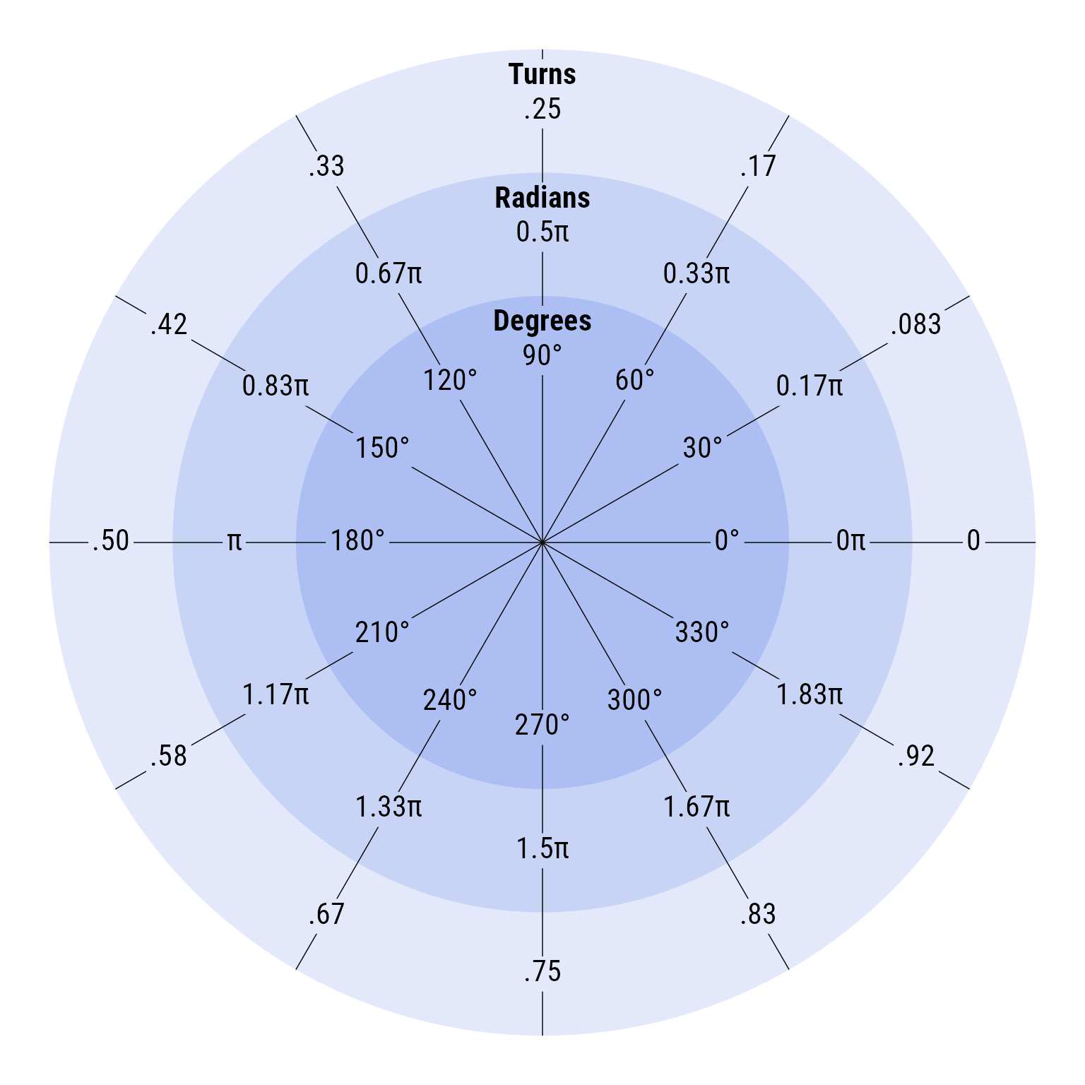

One can create equivalent angles with any of the three metrics.

degree(90)
#> 90°
turn(1 / 4)
#> .25
radian(pi / 2)
#> 0.5π

Although these methods have convenient printing, under the hood they are ob_angle objects can retrieve angle in any of the the three metrics.

radian(pi)
#> π
radian(pi)@degree
#> [1] 180
radian(pi)@turn
#> [1] 0.5

degree(180)
#> 180°
degree(180)@turn
#> [1] 0.5
degree(180)@radian
#> [1] 3.141593

turn(.5)
#> .50
turn(.5)@radian
#> [1] 3.141593
turn(.5)@degree
#> [1] 180

Character Printing

For labeling, sometimes is convenient to convert angles to text:

as.character(degree(90))
#> [1] "90°"
as.character(turn(.25))
#> [1] ".25"
as.character(radian(.5 * pi))
#> [1] "0.5π"

Angle Metric Conversions

Any of the metrics can be converted to any other:

a <- degree(degree = 270)
a
#> 270°
radian(a)
#> 1.5π
turn(a)
#> .75

Arithmetic Operations

Angles can be added, subtracted, multiplied, and divided. The underlying value stored can be any real number (in turn units), but degrees, radians, and turns are always displayed as between −1 and +1 turns, ±360 degrees, or ±2π radians.

30° + 60° = 90°

Code

make_angles <- function(a = c(80, 300), 
                        r = c(.1, .2, .3), 
                        label_adjust = c(0,0,0), 
                        multiplier = c(1.4,1.4,1.4)) {
start_angles <- degree(c(0,a[1], 0))
end_angles <- degree(c(a[1], sum(a), degree(sum(a))@degree))

arc_labels <- as.character(end_angles - start_angles)

mycolors <- c("firebrick4", "royalblue3", "orchid4")


arc_labels[3] <- paste0(arc_labels[1],
                        " + ", 
                        arc_labels[2],
                        " = ", 
                        arc_labels[3])

arcs <- ob_arc(radius = r, 
      start = start_angles, 
      end = end_angles,
      label = ob_label(arc_labels, color = mycolors),
      linewidth = .25,
      length_head = 10,
      arrow_head =  arrowheadr::arrow_head_deltoid(),
      color = mycolors)



ggplot() +
  theme_void() +
  coord_equal()  +
  arcs +
  ob_segment(
    p1 = ob_point(), 
    p2 = ob_polar(theta = degree(c(0,a[1],sum(a))), r = 1), 
    length_head = 5,
    linewidth = .75,
    arrow_head =  arrowheadr::arrow_head_deltoid(),
    color = c("firebrick", "firebrick", "royalblue")) 
}

Code


make_angles(a = c(30, 60), 
            r = c(.12,.24, .36), 
            multiplier = c(1.5,1.5,1.5))

degree(30) + degree(60)
#> 90°

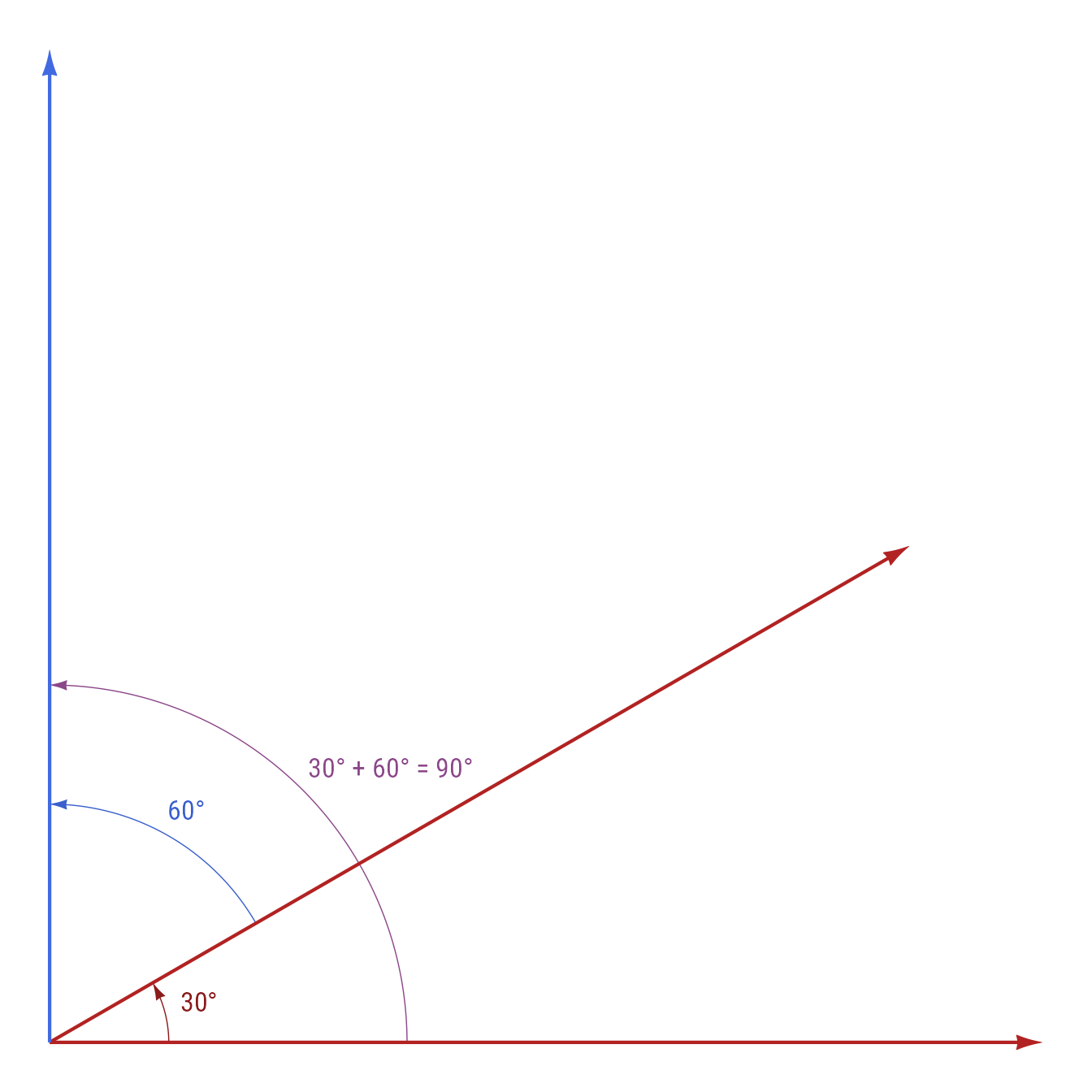
Adding a number to the degree class assumes the number is in the degree metric.

degree(30) + 10
#> 40°

Likewise, adding a number to a radian (or an angle by default) makes a radian:

radian(pi) + 0.5 * pi
#> 1.5π

Turns work the same way:

turn(.1) + .2
#> .30

When degrees are outside the range of ±360, they recalculate:

$\begin{aligned} 80^{\circ} + 300^\circ &= 380^\circ\\ &= 380^\circ-360^\circ\\ &=20^\circ\end{aligned}$

Code

make_angles(c(80, 300))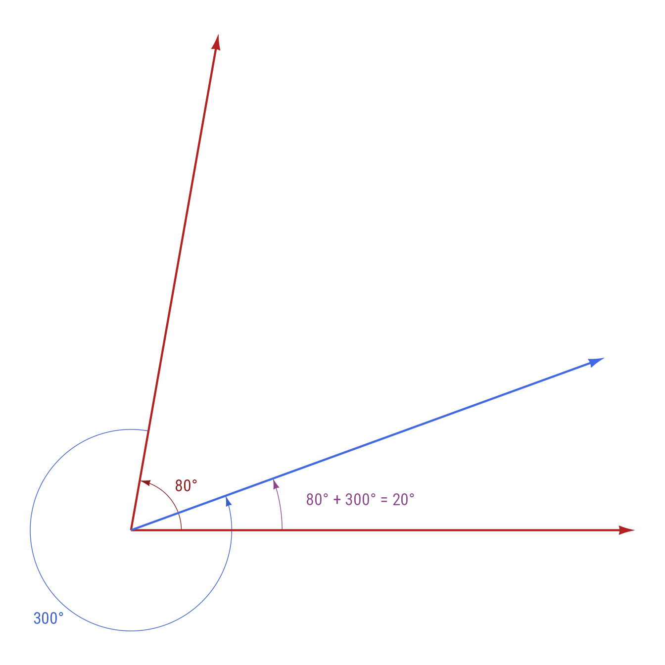

degree(80) + degree(300)
#> 20°

$\begin{aligned} 20^\circ - 40^\circ &= -20^\circ\\&=340^\circ \end{aligned}$

Code

make_angles(c(40, -60))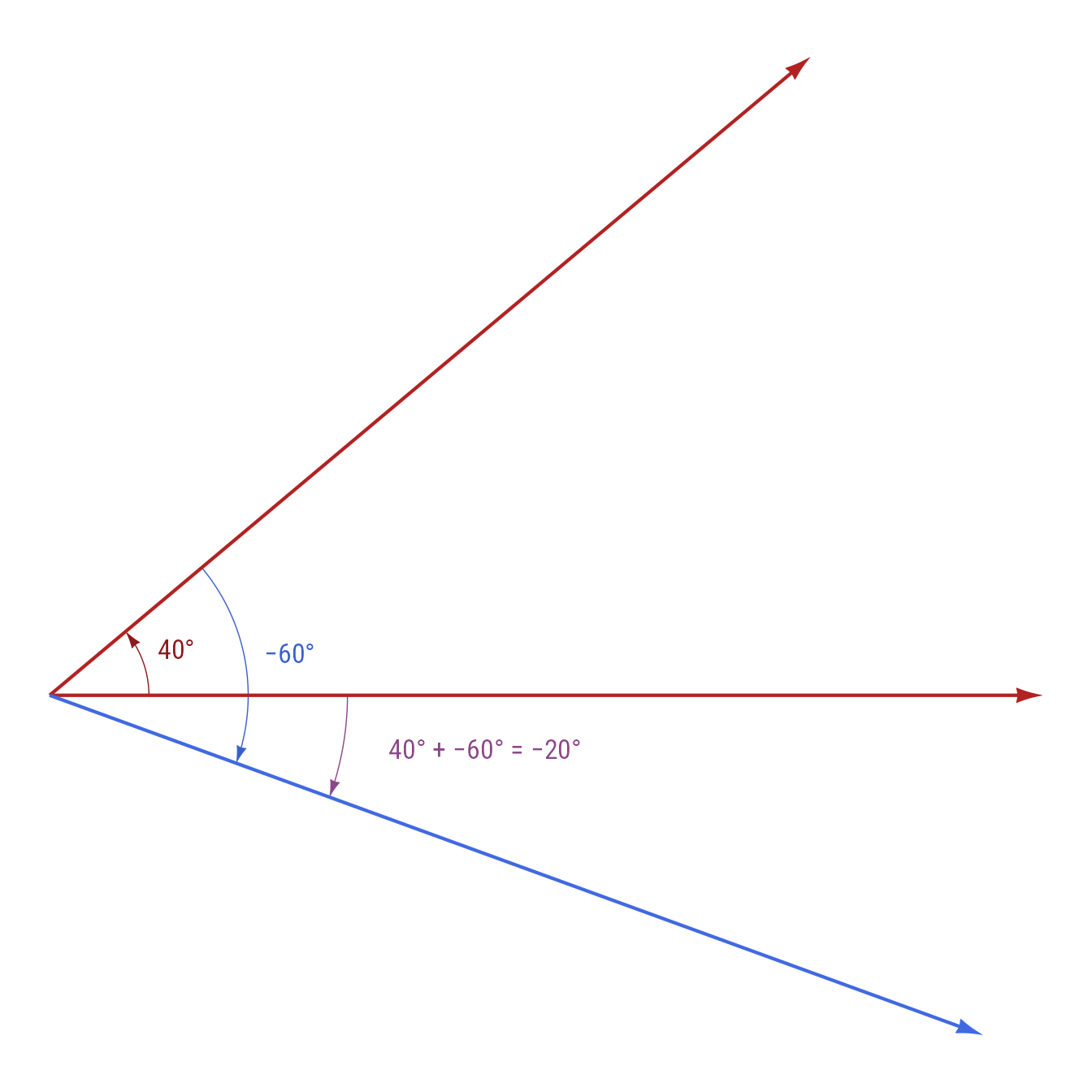

degree(40) - degree(60)
#> −20°

$2\cdot20^\circ=40^\circ$

2 * degree(20)
#> 40°

$\begin{aligned} 2\cdot180 &= 360^\circ\\&=0^\circ \end{aligned}$

2 * degree(180)
#> 0°

Retrieving the underlying data from a `ob_angle` object

Angles created with the degree, radian, or turn function are ob_angle objects. The ob_angle function exists but is not meant to be used directly. Its underlying data is a vector of numeric data representing the number or turns. The underlying turn data from any ob_angle object can be extracted with the c function:

theta <- degree(c(0,180,360, 720))
# Degrees range: 0<= degree < 360
theta@degree
#> [1]   0 180   0   0
# Underlying data in turns
c(theta)
#> [1] 0.0 0.5 1.0 2.0

Trigonometry

Angles can take the three standard trigonometric functions

theta <- degree(60)
cos(theta)
#> [1] 0.5
sin(theta)
#> [1] 0.8660254
tan(theta)
#> [1] 1.732051

Code

o <- ob_point(0, 0)
p <- ob_polar(theta, 1)

# col <- purrr::map2_chr(scico::scico(6, palette = "hawaii"),
#                        c(0.01,0.01,0.01,0.01,.15, .4), 
#                        tinter::darken)

my_colors <- c("#8C0172", "#944046", "#9B7424", 
               "#8EB63B", "#53BD91", "#6C939A")

ggdiagram() +
  ob_circle(fill = NA, color = "gray") +
  # axes
  ob_line(intercept = 0,
       color = "gray",
       linewidth = .25) +
  ob_line(xintercept = 0,
       color = "gray",
       linewidth = .25) +
  # degree arc
  ob_arc(
    end = theta,
    radius = .25,
    label = theta,
    linewidth = .2
  ) +
  # angle arrow
  connect(o, p, label = "*r* = 1", resect_head = 1) +
  # sin(theta)
  ob_segment(
    ob_polar(theta = 0, r = cos(theta)),
    p,
    label = paste0("sin(", 
                   theta,  
                   ") = ", 
                   round(sin(theta), 2)),
    color = my_colors[1],
    linewidth = .5
  ) +
  # cos(theta)
  ob_segment(
    ob_point(0, sin(theta)),
    ob_point(cos(theta), sin(theta)),
    label = ob_label(
      paste0(
        "cos(",
        theta,
        ") = ",
        round(cos(theta), 2)), vjust = 1),
    color = my_colors[2],
    linewidth = .5
  ) +
  # tan(theta)
  ob_segment(
    p,
    p + ob_polar(theta - 90, r = tan(theta)),
    label = paste0(
      "tan(",
      theta,
      ") = ",
      round(tan(theta), 2)),
    color = my_colors[3],
    linewidth = .5
  ) +
  # sec(theta)
  ob_segment(
    o,
    ob_point(1 / cos(theta)),
    label = ob_label(
      label = paste0(
        "sec(",
        theta,
        ") = ",
        round(1 / cos(theta), 2)),
      vjust = 1
    ),
    color = my_colors[5]
  ) +
  # cot(theta)
  ob_segment(
    p + ob_polar(theta + 90, r = 1 / tan(theta)),
    p,
    label = paste0(
      "cot(",
      theta,
      ") = ",
      round(1 / tan(theta), 2)),
    color = my_colors[4],
    linewidth = .5
  ) +
  # csc(theta)
  ob_segment(
    o,
    ob_point(0, 1 / sin(theta)),
    label = paste0(
      "csc(",
      theta,
      ") = ",
      round(1 / sin(theta), 2)),
    color = my_colors[6]
  )

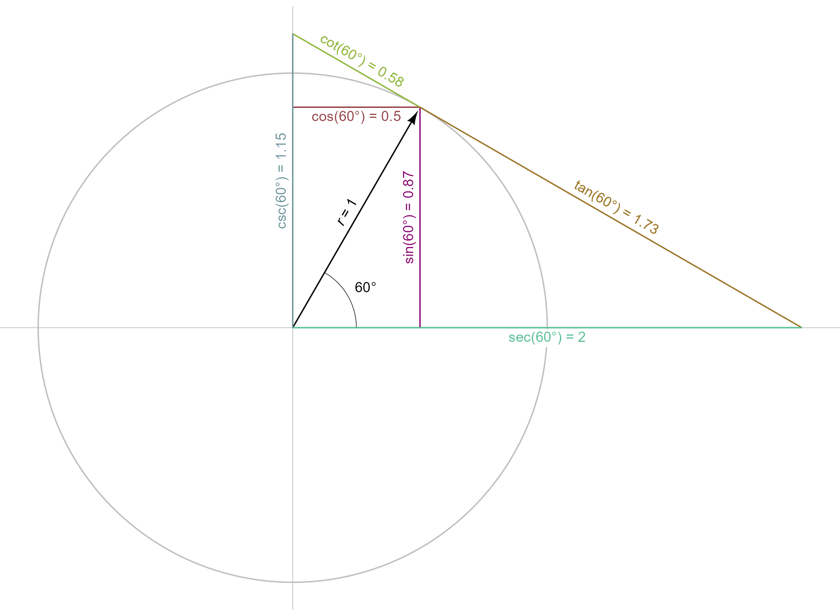
Benefits of using trigonometric functions with angles instead of numeric radians include:

Angle metric conversions are handled automatically.
Under the hood, the cospi, sinpi, and tanpi functions are used to get the rounding right on key locations (e.g., 90 degrees, 180 degrees)

For example, tan(pi) is slightly off from its true value of 0.

tan(pi)
#> [1] -1.224647e-16

By contrast, tan(radian(pi)) rounds to 0 exactly.

tan(radian(pi))
#> [1] 0

Angles

Setup

Angles

Character Printing

Angle Metric Conversions

Arithmetic Operations

Retrieving the underlying data from a ob_angle object

Trigonometry

Retrieving the underlying data from a `ob_angle` object