Setup
Object Lists
Any ggdiagram object made with ob_* functions can be made into a list, either with the list function or the c function.
Binding lists of objects into a single object
The bind function will take a list of the ggdiagram objects and a create single object. If all objects in the list are of a single type (e.g., ob_point), bind will return an object of that type. If the objects are of multiple types, bind will bind each type of object separately and return an ob_shape_list.
Binding objects can make subsequent tasks easier and less repetitive. For example, from the new object p, we can create two circles with one line of code rather than the two lines that would otherwise be needed to create separate circles from p1 and p2.
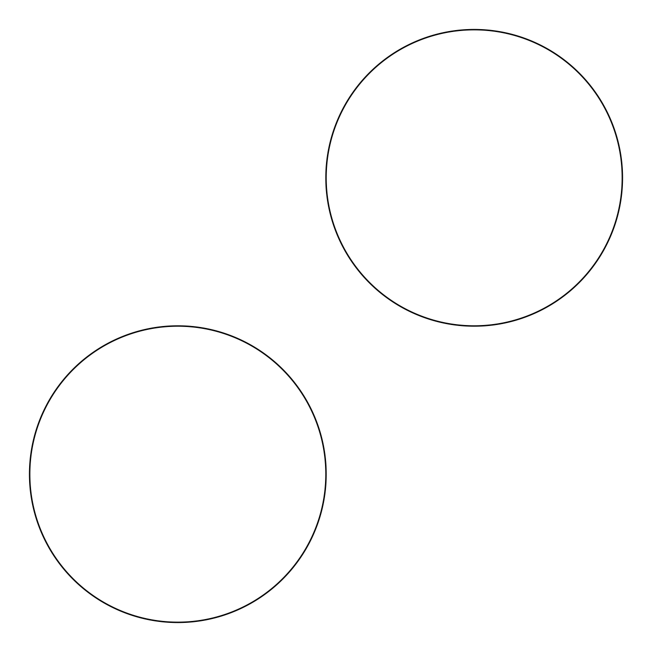
With only two points, the time savings is small. When many objects are bound, the time savings can be substantial.
If the list of objects are of different types, the bind function will bind all objects of the same type and the resulting list will be an ob_shape_list. In Figure 1 we bind 2 points and 2 circles into a ob_shape_list that has 1 ob_point and 1 ob_circle.
p1 <- ob_point(0,0)
p2 <- ob_point(2,0)
c1 <- ob_circle(p1, radius = 2)
c2 <- ob_circle(p2, radius = 1.5)

# bind objectins into an ob_shape_list
osl <- bind(c(p1, p2, c1, c2))
osl
#>
#> ── <ob_shape_list> ─────────────────────────────────────────────────────────────
#>
#> ── <ob_point>
#> # A tibble: 2 × 2
#>       x     y
#>   <dbl> <dbl>
#> 1     0     0
#> 2     2     0
#>
#> ── <ob_circle>
#> # A tibble: 2 × 3
#>       x     y     r
#>   <dbl> <dbl> <dbl>
#> 1     0     0   2
#> 2     2     0   1.5

ggdiagram() +
  osl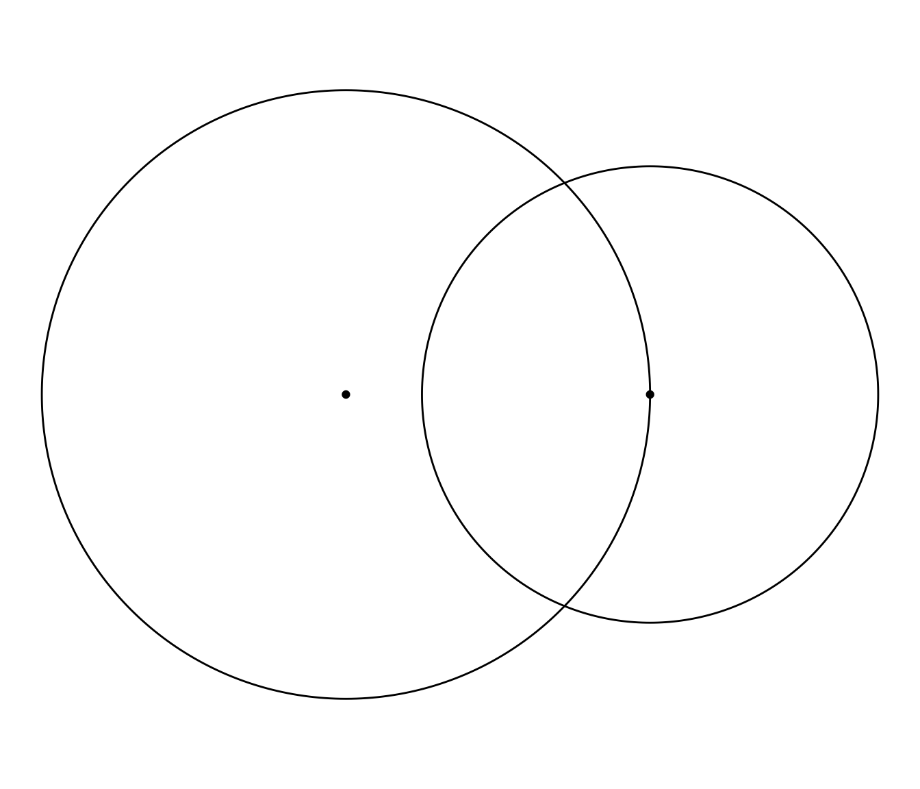
There is not much benefit to making an ob_shape_list as shown here. It would simpler to just include the objects one at a time. However, it can be useful in the context of a large diagram with many elements, each of which would require a separate layer in ggplot2. Binding all the elements first can reduce the number of ggplot layers to the number of object types in the ob_shape_list.
An ob_shape_list’s underlying data is a named list. The names are the functions that were used to create the objects. For example,
osl[["ob_point"]]
#>
#> ── <ob_point>
#> # A tibble: 2 × 2
#>       x     y
#>   <dbl> <dbl>
#> 1     0     0
#> 2     2     0
osl[["ob_circle"]]
#>
#> ── <ob_circle>
#> # A tibble: 2 × 3
#>       x     y     r
#>   <dbl> <dbl> <dbl>
#> 1     0     0   2
#> 2     2     0   1.5
Use unbind to make an object into a list of objects
The unbind function will perform the opposite operation as bind. It converts the elements of an object into a list of singleton objects. For example, object p has two points. Unbinding it will create a list of 2 ob_point objects.
unbind(p)
#> [[1]]
#>
#> ── <ob_point>
#> # A tibble: 1 × 2
#>       x     y
#>   <dbl> <dbl>
#> 1     1     2
#>
#> [[2]]
#>
#> ── <ob_point>
#> # A tibble: 1 × 2
#>       x     y
#>   <dbl> <dbl>
#> 1     3     4
The unbind function is needed when we want to loop through each element using lapply or purrr::map. In Figure 2, we have three points arranged in an equilateral triangle. We unbind the points so that we can use map to place three points around each point. Each point is then plotted as triangles. To make the list something that ggplot2 can plot, we can bind the list into a single object.
theta <- degree(seq(90, 360, 120))
ggdiagram() +
  {p_3 <- ob_polar(
        theta = theta,
        r = .5,
        fill = "black",
        shape = "triangle down filled",
        size = 15)} +
  unbind(p_3) %>%
    purrr::map(
      \(p_i) {
        p_i + ob_polar(
          theta = theta,
          r = .15,
          color = "orchid",
          fill = "orchid",
          size = 15,
          shape = "triangle filled")}) %>%
  bind() +
  scale_x_continuous(NULL, expand = expansion(.15))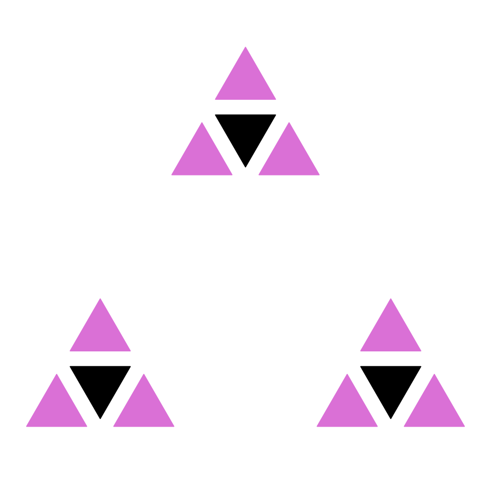
unbind, map, and bind to loop through elements.
Alternatively, we can convert each list item into a geom with as.geom as in Figure 3.
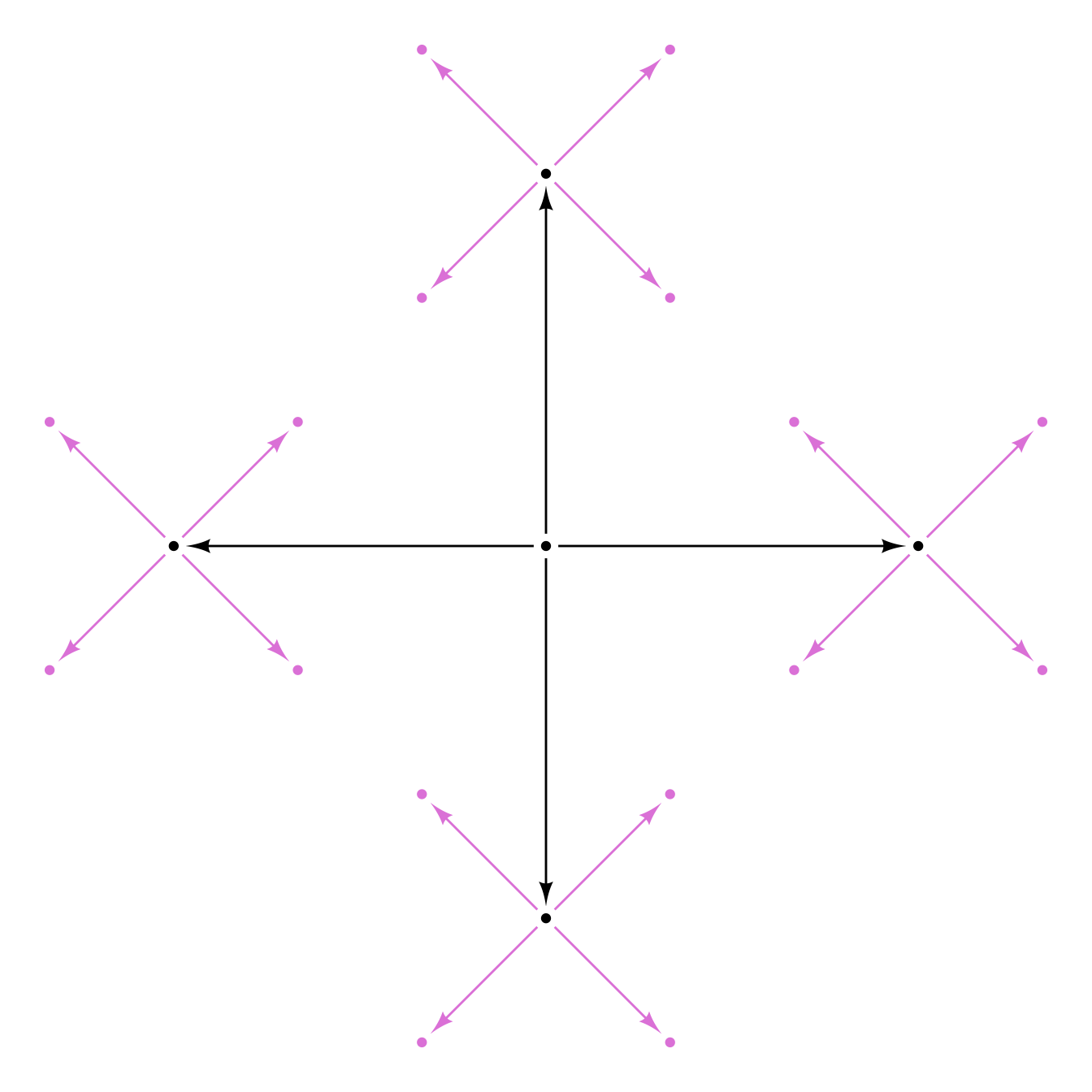
Use map_ob to loop through object elements
To unbind, map, and then bind can be tedious every time a loop is needed. The map_ob function is a wrapper for map that unbinds the input and binds the output automatically.
ggdiagram() +
  {o <- ob_point()} +
  {p <- ob_polar(degree(c(0, 90, 180, 270)))} +
  connect(o, p, resect = 2) +
  p %>%
    map_ob(\(pp) {
      p2 <- pp + ob_polar(theta = degree(seq(45, 315, 90)),
                          r = sqrt(2) / 3,
                          color = "orchid")
      list(p2,
           connect(pp, p2, resect = 2))
}) 
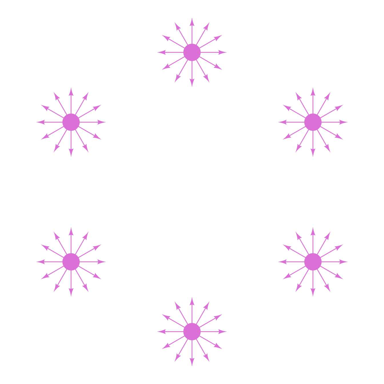
The ob_map function can output a list of different object types simultaneously.
theta <- degree(seq(0,300, 60))

ggdiagram() +
  {e6 <- ob_ellipse(
    center = ob_polar(
      theta = theta,
      r = 60),
    m1 = .5,
    a = 8,
    b = 4,
    angle = theta + degree(90),
    color = NA,
    fill = "orchid4",
    size = 4)} +
  map_ob(e6, \(e_i) {
    p_i <- e_i@center
    p_ij <- p_i + ob_polar(theta, 15)
    c_ij <- ob_circle(
      center = p_ij,
      radius = 2,
      fill = "green4",
      color = NA)
    p_ijk <- map_ob(p_ij, \(pt_ij) {
      ob_segment(pt_ij, pt_ij + ob_polar(theta, 4) )
      })
    list(p_ijk, c_ij)
  })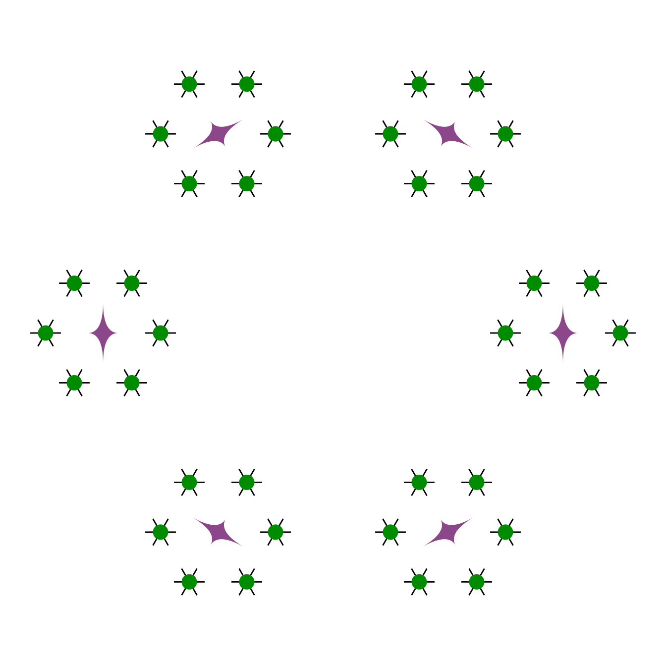
map_ob.
In a more practical example, every variable in the left column of Figure 6 is connected to every variable on the right.
k <- 5
clr <- viridis::viridis(k, begin = .3, end = .7)
ggdiagram() +
  {t1 <- ob_array(ob_circle(), k = k, where = "north",
                  fill = clr,
                  color = clr)} +
  {t2 <- ob_circle(fill = clr, color = clr)@place(
    from = t1,
    where = "right",
    sep = 10)} +
  map_ob(t1, \(tt) {
    connect(tt, t2, resect = 2, color = tt@color)
  })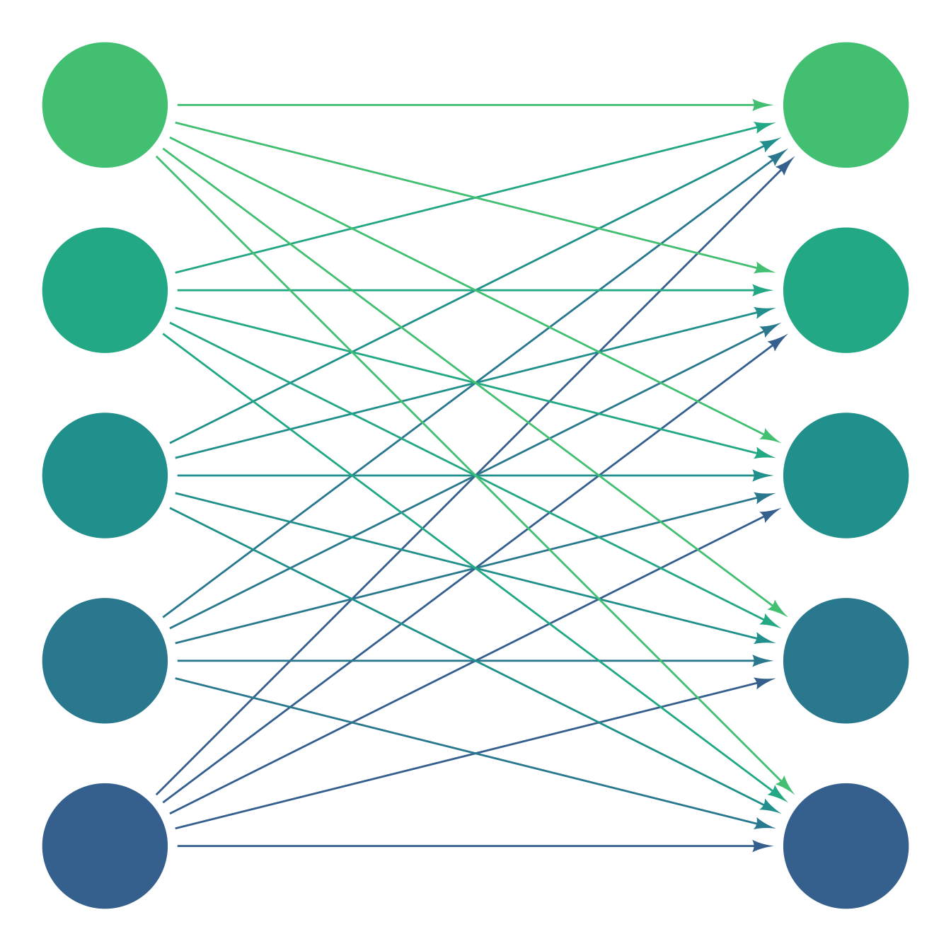
map_ob to the connect variables
Subsetting objects
The [ operator can subset ggdiagram objects created with ob_* functions. Object p has 2 points in it. To select the first point only:
p[1]
#>
#> ── <ob_point>
#> # A tibble: 1 × 2
#>       x     y
#>   <dbl> <dbl>
#> 1     1     0
The strategic use of subsetting can make otherwise repetitive tasks much less tedious. In Figure 7, we connect a ring of 12 circles with one command rather than 12.
theta <- degree(seq(0,330,30))
clr <- hsv(theta@degree / 360, s = .4, v = .6)
ggdiagram() +
  {c12 <- ob_circle(
    center = ob_polar(theta, r = 6),
    fill = clr,
    color = NA)} +
  connect(c12, c12[c(2:12, 1)],
          resect = 2,
color = clr) 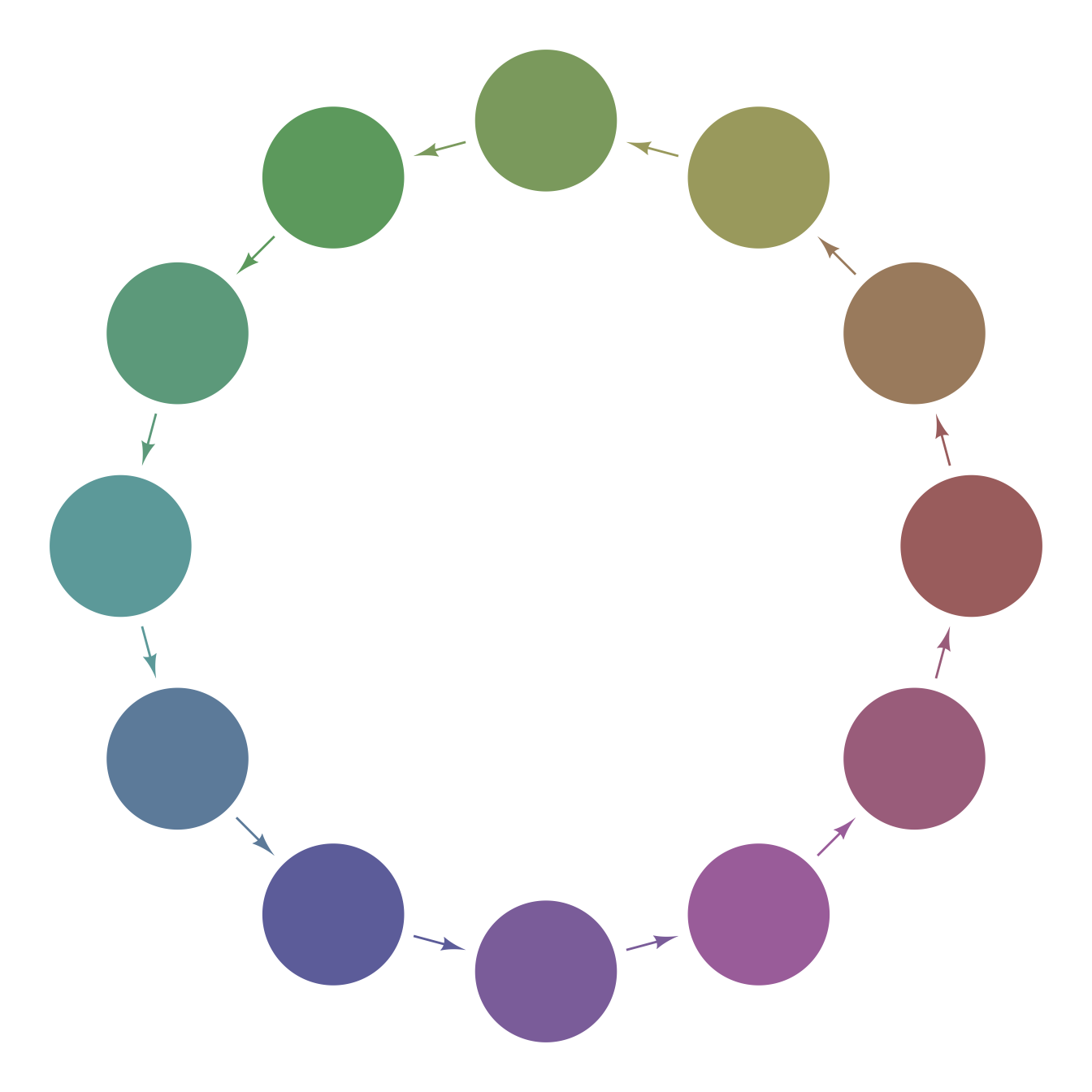
Subsetting can be used for assignment in ggdiagram objects. For example, in Figure 8, the first of four points is changed from (1,5) to (0,0)
p <- ob_point(x = 1:4,
              y = 2:5)
p[1] <- ob_point(0,0, color = "firebrick", size = 5)

ggplot() +
  coord_equal() +
p 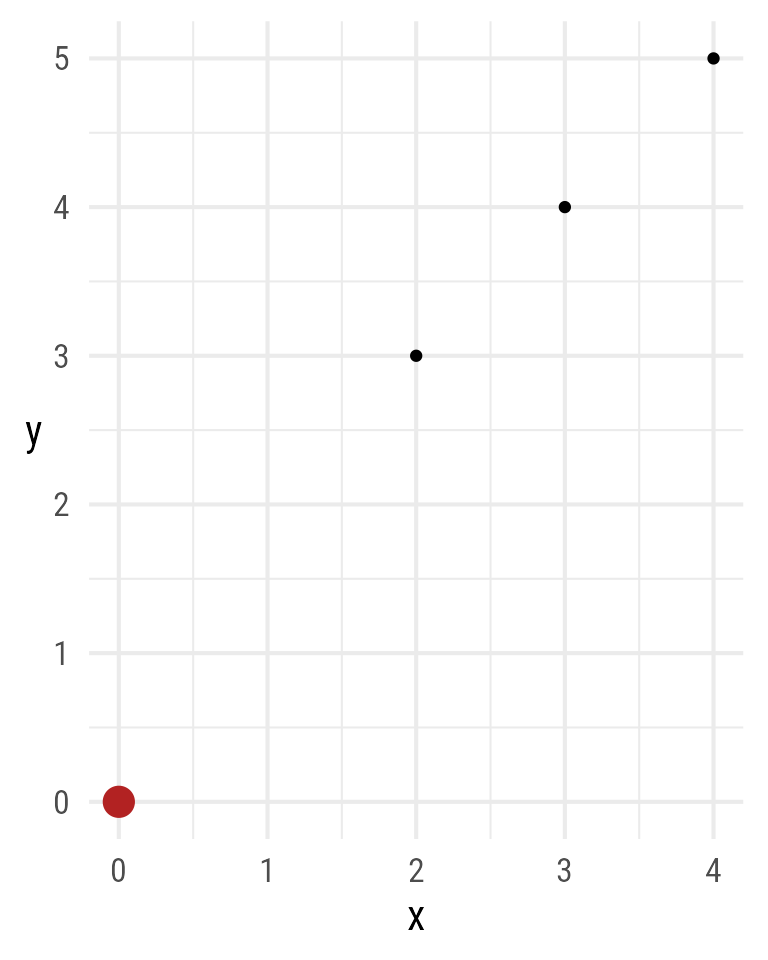
In Figure 9, there are 8 variables with 13 arrows connecting them. Rather than making a separate connection for each arrow, subsetting allows us to make all 13 connections with a single connect command. Using subsetting to assign variables within a for loop allows for placing the variables programmatically. If more or fewer variables are desired, setting k to another value, will create k variables and 2k − 3 connections.
# Number of variables
k <- 8L

# Make k variables
x <- ob_rectangle(ob_point(rep(0, k), rep(0, k)),
                  label = ob_label(
                    label = paste0("*X*~", 1:k, "~"),
                    vjust = .6,
                    size = 20,
                    family = "Roboto Condensed"
                  ))


# Place even variables to the right and
# odd variables below the previous variables
for (i in 2:k) {
  x[i] <- place(x[i], x[i - 1], ifelse((i %% 2) == 0, "right", "below"))
}

# Plot
ggdiagram() +
  x +
  # paths between variables ahead by 1 and by 2
  connect(x[c(seq(1,k - 1), seq(1, k - 2))],
          x[c(seq(2,k),     seq(3, k))],
          resect = 2)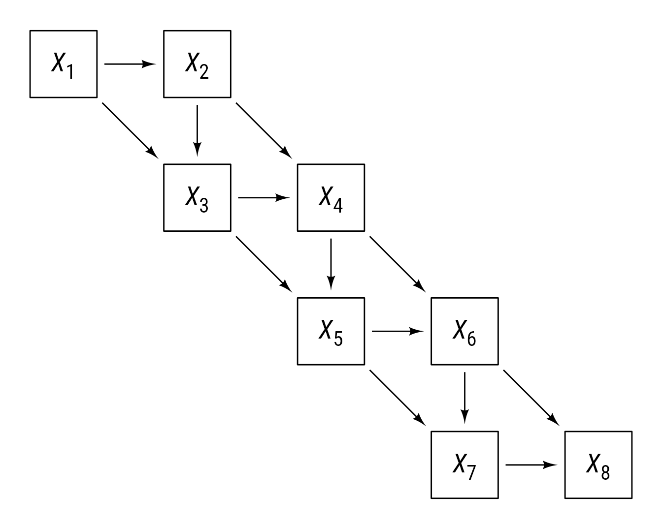
Subset by id
Functions with an ob_* prefix have an id property that can be used to subset objects. The id property does not have to be unique.
Creating objects from data.frames/tibbles
The data2shape function will convert a data.frame (or tibble) to a ggdiagram ob_... function. For example, Figure 10, a sequence of regular polygons was quickly and efficiently.
d <- tibble(
  x = 3:10,
  y = x,
  alpha = x * .1,
  radius = .6,
  angle = 90,
  fill = "dodgerblue4",
  n = x
)

ggdiagram() +
  data2shape(data = d, shape = ob_ngon)
Although data2shape is sometimes less verbose than standard ggplot2 syntax, using it is not always the best choice. If you start with a data.frame (or tibble), and all you need to do is display data, the standard ggplot2 functions are optimized for this purpose, particularly when the data set is large. In general, the direct use of a ggplot2 function will render more quickly than its analogous ggdiagram function. The reason to convert data to shapes via data2shape is to do something that would be otherwise difficult with the standard ggplot2 functions.
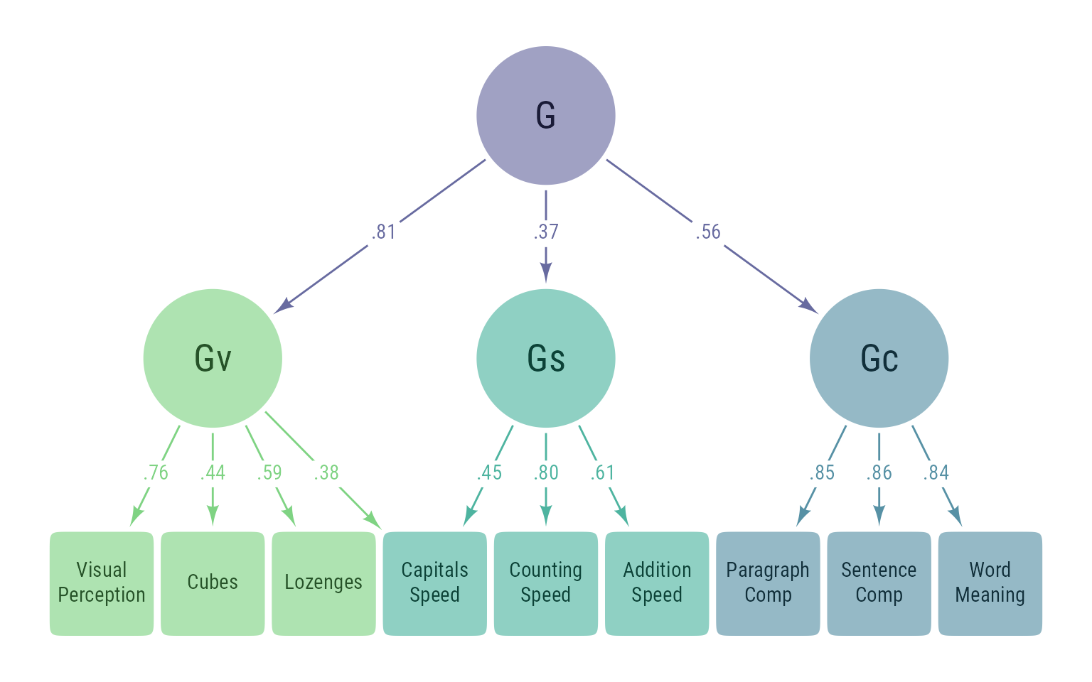
For example, one of the problems that prompted me to make the ggdiagram package was that I wanted to make path diagrams for structural equation models with full control of every aspect of the diagram. There are excellent functions from other packages that automate the process of making a path diagram (e.g., semPlot, semptools, and lavaanPlot), with options for greater flexibility. Even so, I could not figure out how to make the plots fully customizable.
My eventual goal is for ggdiagram to automate the tedious parts of making path diagrams and allow for efficient customization. The code for Figure 11 shows the whole process, including the tedious bits that eventually will be tucked way in functions.
library(dplyr)
library(tidyr)
library(lavaan)

# Observed variable name conversion
onames <- c(VisualPerception = "x1",
               Cubes = "x2",
               Lozenges = "x3",
               CapitalsSpeed = "x9",
               AdditionSpeed = "x7",
               CountingSpeed = "x8",
               ParagraphComp = "x4",
               SentenceComp = "x5",
               WordMeaning = "x6")

# Data
d <- lavaan::HolzingerSwineford1939 |>
  dplyr::select(x1:x9) |>
  dplyr::rename(all_of(onames))

# Structural Model
m <- '
Gv =~ VisualPerception + Cubes + Lozenges + CapitalsSpeed
Gs =~ CapitalsSpeed + CountingSpeed + AdditionSpeed
Gc =~ ParagraphComp + SentenceComp + WordMeaning
g =~ Gv + Gc + Gs
'

# Fit model with converted names
fit <- sem(m, data = d)

# Parameter table, find primary indicators
pt <- standardizedsolution(fit) %>%
  mutate(primary_indicator = dplyr::dense_rank(
    desc(abs(est.std))) == 1 & op == "=~",
    .by = c(rhs, op))

# Oberved and latent names
o_names <- lavaan::lavNames(fit, "ov")
l_names <- lavaan::lavNames(fit, "lv")

# Make colors
latent_colors <- l_names %>%
  length() %>%
  viridis::viridis(alpha = .5, begin = .2, end = .75) %>%
  `names<-`(rev(l_names))

# Make data for creating objects
d <- tibble(id = c(o_names, l_names))  %>%
  mutate(depth = get_depth(id, model = m),
         type = ifelse(id %in% l_names, "latent", "observed"),
         m1 = ifelse(type == "latent", 2, 15),
         a = ifelse(type == "latent", 2, 1.5),
         color = NA,
         indicators = map(id, \(v) {
           pt %>%
             filter(op == "=~" & lhs == v) %>%
             select(indicator = rhs,
                    loading = est.std,
                    primary_indicator)
         }),
         dvs = map(id, \(v) {
           pt %>%
             filter(op == "~" & rhs == v) %>%
             select(dv = rhs,
                    b = est.std)
         }),
         parents = map(id, \(v) {
           pt %>%
             filter(op == "=~" & rhs == v) %>%
             arrange(desc(abs(est.std))) %>%
             pull(lhs)
         }),
         fill = pmap_chr(
           list(i = id,
                tp = type,
                prnts = parents),
           function(i, tp, prnts) {
             if (tp == "latent") {
               fll <- latent_colors[i ]
             } else {
               fll <- latent_colors[prnts[1]]

             }
             fll
           })) %>%
  mutate(
    label = snakecase::to_title_case(id) %>%
      stringr::str_wrap(width = 10,
                        whitespace_only = FALSE) %>%
      stringr::str_replace_all(pattern = "\\n", "<br>")) %>%
  arrange(depth)

# Make shapes
s <- data2shape(d, ob_ellipse)

# Format shape labels
s@label@size[d$type == "latent"] <- 20
s@label@nudge_y[d$type == "latent"] <- -0.08
s@label@color <- class_color(s@fill)@darken(.6)@color

# Position shapes:
#   Move indicators to the right of other indicators
#   Center latent variables above their primary indicators
walk(d$id, \(v) {
  dr <- d %>% filter(id == v)

  children <- dr %>%
    unnest(indicators) %>%
    filter(primary_indicator) %>%
    pull(indicator)

  if (pull(dr, depth) == 1) {
    s[v] <<- place(s[v],
                   s@bounding_box,
                   "right",
                   sep = .2)
  } else {
    s[v] <<- place(s[v],
                   s[children]@bounding_box@north,
                   "above",
                   sep = 4)
  }

})

# Make edges
e <- d %>%
  unnest(indicators) %>%
  select(id, indicator, loading, fill) %>%
  nest(.by = id) %>%
  pmap(\(id, data) {

    children <- pull(data, indicator)
    ll <- pull(data, loading) %>%
      round_probability()

    connect(from = s[id],
            to = s[children],
            # to_offset = ob_point(0,4),
            label = ob_label(ll, angle = 0, position = .47),
            label_sloped = F,
            resect = 1,
            color = class_color(data$fill)@lighten(.8)
            )@set_label_y()

  }) %>%
  bind()

# Make plot
ggdiagram(font_family = my_font,
          font_size = 12) +
  s +
  e